Hands-on Exercise 1A: Geospatial Data Wrangling with R

Author

Kristine Joy Paas

Published

November 16, 2023

Modified

November 19, 2023

Overview

This hands-on exercise covers Chapter 1: Data Wrangling with R.

I learned about the following:

Public Data Sets like the ones on data.gov.sg, LTADataMall, and InsideAirbnb.
How to import data sets into RStudio
Wrangling geospatial data in using different R packages like sf, tidyverse, etc.
Creating thematic/choropleth maps with tmap

Getting Started

Preparing the data sets

First, I downloaded the different data sets needed in this exercise.

Geospatial

Master Plan 2014 Subzone Boundary (Web) from data.gov.sg
Pre-Schools Location from data.gov.sg
Cycling Path from LTADataMall

Aspatial

Latest version of Singapore Airbnb listing data from Inside Airbnb

Next, is putting them under the Hands-on_Ex1 directory, with the following file structure:

Hands-on_Ex1
└── data
    ├── aspatial
    │   └── listings.csv
    └── geospatial
        ├── CyclingPathGazette.cpg
        ├── CyclingPathGazette.dbf
        ├── CyclingPathGazette.lyr
        ├── CyclingPathGazette.prj
        ├── CyclingPathGazette.sbn
        ├── CyclingPathGazette.sbx
        ├── CyclingPathGazette.shp
        ├── CyclingPathGazette.shp.xml
        ├── CyclingPathGazette.shx
        ├── MP14_SUBZONE_WEB_PL.dbf
        ├── MP14_SUBZONE_WEB_PL.prj
        ├── MP14_SUBZONE_WEB_PL.sbn
        ├── MP14_SUBZONE_WEB_PL.sbx
        ├── MP14_SUBZONE_WEB_PL.shp
        ├── MP14_SUBZONE_WEB_PL.shp.xml
        ├── MP14_SUBZONE_WEB_PL.shx
        └── PreSchoolsLocation.kml

Installing R packages

I used the code below to install the R packages used in the exercise:

pacman::p_load(sf, tidyverse)

Importing Geospatial Data

After setting up the data sets and the R packages, we can proceed with importing the geospatial data.

Master Plan 2014 Subzone Boundary (Web)

To import the data set to RStudio, I used st_read() :

mpsz <- st_read(dsn = "data/geospatial", layer = "MP14_SUBZONE_WEB_PL")

Reading layer `MP14_SUBZONE_WEB_PL' from data source 
  `/Users/kjcpaas/Documents/Grad School/ISSS624/Project/ISSS624/Hands-on_Ex1/data/geospatial' 
  using driver `ESRI Shapefile'
Simple feature collection with 323 features and 15 fields
Geometry type: MULTIPOLYGON
Dimension:     XY
Bounding box:  xmin: 2667.538 ymin: 15748.72 xmax: 56396.44 ymax: 50256.33
Projected CRS: SVY21

I encountered the error below along the way:

Cannot open layer MasterPlan2014SubzoneBoundaryWebKML

This is because I originally downloaded the kml file instead of the shp file. After using the shp file, the st_read() succeeded.

ℹ️ My biggest take-away for this is that st_read reads shp data set by default. (this would be debunked later)

After running the code, we should see the mpsz data in the environment.

Cycling Path Data

Equipped with my learning from the previous step, I was able to quickly figure out that importing this data set can be done by simply changing the layer parameter from the previous code:

cyclingpath <- st_read(dsn = "data/geospatial", layer = "CyclingPathGazette")

Reading layer `CyclingPathGazette' from data source 
  `/Users/kjcpaas/Documents/Grad School/ISSS624/Project/ISSS624/Hands-on_Ex1/data/geospatial' 
  using driver `ESRI Shapefile'
Simple feature collection with 2558 features and 2 fields
Geometry type: MULTILINESTRING
Dimension:     XY
Bounding box:  xmin: 11854.32 ymin: 28347.98 xmax: 42626.09 ymax: 48948.15
Projected CRS: SVY21

However, the difference is that this geometry has polyline features, while the previous has polygon features.

Pre-Schools Location Data

Unlike the others, this data set is in kml format instead of shp format. I used the following code to import:

preschool <- st_read("data/geospatial/PreSchoolsLocation.kml")

Reading layer `PRESCHOOLS_LOCATION' from data source 
  `/Users/kjcpaas/Documents/Grad School/ISSS624/Project/ISSS624/Hands-on_Ex1/data/geospatial/PreSchoolsLocation.kml' 
  using driver `KML'
Simple feature collection with 2290 features and 2 fields
Geometry type: POINT
Dimension:     XYZ
Bounding box:  xmin: 103.6878 ymin: 1.247759 xmax: 103.9897 ymax: 1.462134
z_range:       zmin: 0 zmax: 0
Geodetic CRS:  WGS 84

ℹ️ Contrary to my previous take-away, st_read() can read kml files by default. In fact, reading shp files require more parameters like dsn and layer.

Checking Contents of Data Frames

Checking the geometry of data frames

Using st_geometry() returns information about the geometry of the data frame.

st_geometry(mpsz)

Geometry set for 323 features 
Geometry type: MULTIPOLYGON
Dimension:     XY
Bounding box:  xmin: 2667.538 ymin: 15748.72 xmax: 56396.44 ymax: 50256.33
Projected CRS: SVY21
First 5 geometries:

It gave the same geometric information as when importing the shape data but with additional details like the first 5 geometries.

Getting overview of geospatial data

Using glimpse() gives useful information about the columns, data types, values. For example:

glimpse(mpsz)

Rows: 323
Columns: 16
$ OBJECTID   <int> 1, 2, 3, 4, 5, 6, 7, 8, 9, 10, 11, 12, 13, 14, 15, 16, 17, …
$ SUBZONE_NO <int> 1, 1, 3, 8, 3, 7, 9, 2, 13, 7, 12, 6, 1, 5, 1, 1, 3, 2, 2, …
$ SUBZONE_N  <chr> "MARINA SOUTH", "PEARL'S HILL", "BOAT QUAY", "HENDERSON HIL…
$ SUBZONE_C  <chr> "MSSZ01", "OTSZ01", "SRSZ03", "BMSZ08", "BMSZ03", "BMSZ07",…
$ CA_IND     <chr> "Y", "Y", "Y", "N", "N", "N", "N", "Y", "N", "N", "N", "N",…
$ PLN_AREA_N <chr> "MARINA SOUTH", "OUTRAM", "SINGAPORE RIVER", "BUKIT MERAH",…
$ PLN_AREA_C <chr> "MS", "OT", "SR", "BM", "BM", "BM", "BM", "SR", "QT", "QT",…
$ REGION_N   <chr> "CENTRAL REGION", "CENTRAL REGION", "CENTRAL REGION", "CENT…
$ REGION_C   <chr> "CR", "CR", "CR", "CR", "CR", "CR", "CR", "CR", "CR", "CR",…
$ INC_CRC    <chr> "5ED7EB253F99252E", "8C7149B9EB32EEFC", "C35FEFF02B13E0E5",…
$ FMEL_UPD_D <date> 2014-12-05, 2014-12-05, 2014-12-05, 2014-12-05, 2014-12-05…
$ X_ADDR     <dbl> 31595.84, 28679.06, 29654.96, 26782.83, 26201.96, 25358.82,…
$ Y_ADDR     <dbl> 29220.19, 29782.05, 29974.66, 29933.77, 30005.70, 29991.38,…
$ SHAPE_Leng <dbl> 5267.381, 3506.107, 1740.926, 3313.625, 2825.594, 4428.913,…
$ SHAPE_Area <dbl> 1630379.27, 559816.25, 160807.50, 595428.89, 387429.44, 103…
$ geometry   <MULTIPOLYGON [m]> MULTIPOLYGON (((31495.56 30..., MULTIPOLYGON (…

This will be very useful to scan for the available data and which columns are useful for analysis.

Revealing complete information of feature objects

Using head() can give full information about objects in the data set. For example:

head(mpsz, n=5)

Simple feature collection with 5 features and 15 fields
Geometry type: MULTIPOLYGON
Dimension:     XY
Bounding box:  xmin: 25867.68 ymin: 28369.47 xmax: 32362.39 ymax: 30435.54
Projected CRS: SVY21
  OBJECTID SUBZONE_NO      SUBZONE_N SUBZONE_C CA_IND      PLN_AREA_N
1        1          1   MARINA SOUTH    MSSZ01      Y    MARINA SOUTH
2        2          1   PEARL'S HILL    OTSZ01      Y          OUTRAM
3        3          3      BOAT QUAY    SRSZ03      Y SINGAPORE RIVER
4        4          8 HENDERSON HILL    BMSZ08      N     BUKIT MERAH
5        5          3        REDHILL    BMSZ03      N     BUKIT MERAH
  PLN_AREA_C       REGION_N REGION_C          INC_CRC FMEL_UPD_D   X_ADDR
1         MS CENTRAL REGION       CR 5ED7EB253F99252E 2014-12-05 31595.84
2         OT CENTRAL REGION       CR 8C7149B9EB32EEFC 2014-12-05 28679.06
3         SR CENTRAL REGION       CR C35FEFF02B13E0E5 2014-12-05 29654.96
4         BM CENTRAL REGION       CR 3775D82C5DDBEFBD 2014-12-05 26782.83
5         BM CENTRAL REGION       CR 85D9ABEF0A40678F 2014-12-05 26201.96
    Y_ADDR SHAPE_Leng SHAPE_Area                       geometry
1 29220.19   5267.381  1630379.3 MULTIPOLYGON (((31495.56 30...
2 29782.05   3506.107   559816.2 MULTIPOLYGON (((29092.28 30...
3 29974.66   1740.926   160807.5 MULTIPOLYGON (((29932.33 29...
4 29933.77   3313.625   595428.9 MULTIPOLYGON (((27131.28 30...
5 30005.70   2825.594   387429.4 MULTIPOLYGON (((26451.03 30...

This will return the first 5 objects, and the number of objects can be set by specifying a value for n.

Another function that is useful for this purpose is tail(), which returns items from the end of the data set. For example:

tail(mpsz, n=2)

Simple feature collection with 2 features and 15 fields
Geometry type: MULTIPOLYGON
Dimension:     XY
Bounding box:  xmin: 23378.74 ymin: 48569.62 xmax: 28343.2 ymax: 50256.33
Projected CRS: SVY21
    OBJECTID SUBZONE_NO    SUBZONE_N SUBZONE_C CA_IND PLN_AREA_N PLN_AREA_C
322      322          7  THE WHARVES    SBSZ07      N  SEMBAWANG         SB
323      323          8 SENOKO NORTH    SBSZ08      N  SEMBAWANG         SB
        REGION_N REGION_C          INC_CRC FMEL_UPD_D   X_ADDR   Y_ADDR
322 NORTH REGION       NR 6D89875A351CF51C 2014-12-05 26945.07 49552.79
323 NORTH REGION       NR A800CBEE879C1BF9 2014-12-05 24665.79 49482.60
    SHAPE_Leng SHAPE_Area                       geometry
322  11828.878    1635808 MULTIPOLYGON (((26219.89 50...
323   7392.129    2241387 MULTIPOLYGON (((26047.11 50...

This returned the items on rows 322 and 323 instead of 1 and 2 if we were to use head().

However, I wonder which use cases these functions would be useful as we can easily inspect the full data when looking at all the Environment Data in RStudio. 🤔

Plotting Geospatial Data

plot(mpsz, max.plot = 15)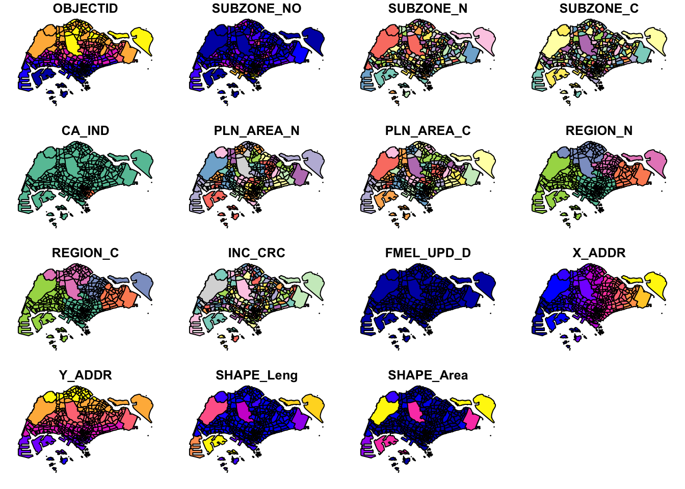

I was pleasantly surprised to find that the rendering of the plots was so fast! It only took 1 second or so on my machine for 300+ features and 15 fields. This is really useful for quick look of the data.

Trying it on the cycling path data was also very fast though the result was not so useful for me as it needs to be overlayed with a map like above.

plot(cyclingpath)

I wonder how long it would take once we have larger data sets. 🤔

As someone not originally from Singapore, I am still familiarizing myself with the countries geography so I’ll plot the regions first.

plot(mpsz['REGION_N'])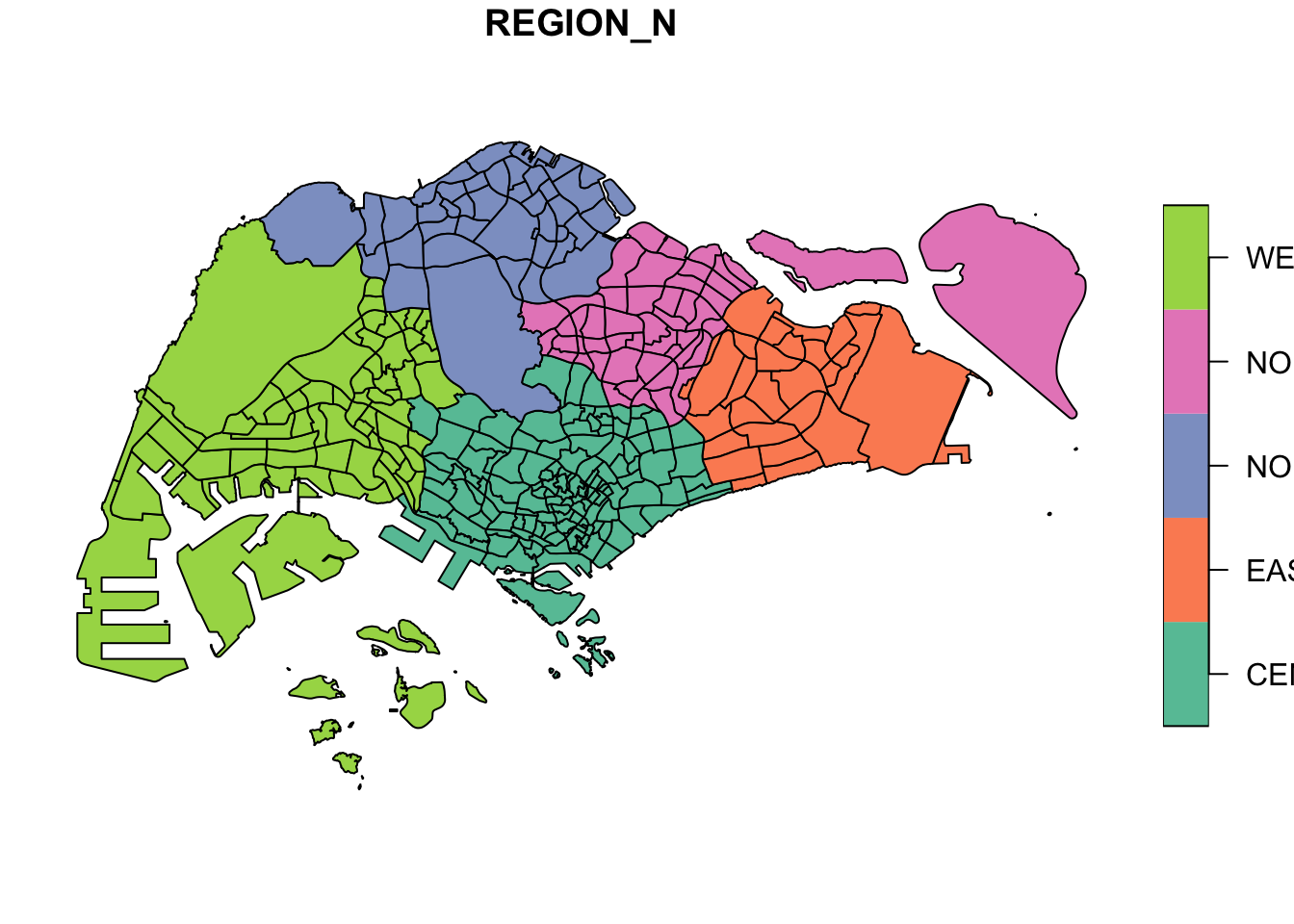

This can still be visualized better, especially the names in the legend got cut off. From the Help pages on RStudio, this function has a lot more parameters and I’ll explore it once I have more time.

Projections

Correcting the EPSG code

st_crs(mpsz)

Coordinate Reference System:
  User input: SVY21 
  wkt:
PROJCRS["SVY21",
    BASEGEOGCRS["SVY21[WGS84]",
        DATUM["World Geodetic System 1984",
            ELLIPSOID["WGS 84",6378137,298.257223563,
                LENGTHUNIT["metre",1]],
            ID["EPSG",6326]],
        PRIMEM["Greenwich",0,
            ANGLEUNIT["Degree",0.0174532925199433]]],
    CONVERSION["unnamed",
        METHOD["Transverse Mercator",
            ID["EPSG",9807]],
        PARAMETER["Latitude of natural origin",1.36666666666667,
            ANGLEUNIT["Degree",0.0174532925199433],
            ID["EPSG",8801]],
        PARAMETER["Longitude of natural origin",103.833333333333,
            ANGLEUNIT["Degree",0.0174532925199433],
            ID["EPSG",8802]],
        PARAMETER["Scale factor at natural origin",1,
            SCALEUNIT["unity",1],
            ID["EPSG",8805]],
        PARAMETER["False easting",28001.642,
            LENGTHUNIT["metre",1],
            ID["EPSG",8806]],
        PARAMETER["False northing",38744.572,
            LENGTHUNIT["metre",1],
            ID["EPSG",8807]]],
    CS[Cartesian,2],
        AXIS["(E)",east,
            ORDER[1],
            LENGTHUNIT["metre",1,
                ID["EPSG",9001]]],
        AXIS["(N)",north,
            ORDER[2],
            LENGTHUNIT["metre",1,
                ID["EPSG",9001]]]]

mpsz3414 <- st_set_crs(mpsz, 3414)

st_crs(mpsz3414)

Coordinate Reference System:
  User input: EPSG:3414 
  wkt:
PROJCRS["SVY21 / Singapore TM",
    BASEGEOGCRS["SVY21",
        DATUM["SVY21",
            ELLIPSOID["WGS 84",6378137,298.257223563,
                LENGTHUNIT["metre",1]]],
        PRIMEM["Greenwich",0,
            ANGLEUNIT["degree",0.0174532925199433]],
        ID["EPSG",4757]],
    CONVERSION["Singapore Transverse Mercator",
        METHOD["Transverse Mercator",
            ID["EPSG",9807]],
        PARAMETER["Latitude of natural origin",1.36666666666667,
            ANGLEUNIT["degree",0.0174532925199433],
            ID["EPSG",8801]],
        PARAMETER["Longitude of natural origin",103.833333333333,
            ANGLEUNIT["degree",0.0174532925199433],
            ID["EPSG",8802]],
        PARAMETER["Scale factor at natural origin",1,
            SCALEUNIT["unity",1],
            ID["EPSG",8805]],
        PARAMETER["False easting",28001.642,
            LENGTHUNIT["metre",1],
            ID["EPSG",8806]],
        PARAMETER["False northing",38744.572,
            LENGTHUNIT["metre",1],
            ID["EPSG",8807]]],
    CS[Cartesian,2],
        AXIS["northing (N)",north,
            ORDER[1],
            LENGTHUNIT["metre",1]],
        AXIS["easting (E)",east,
            ORDER[2],
            LENGTHUNIT["metre",1]],
    USAGE[
        SCOPE["Cadastre, engineering survey, topographic mapping."],
        AREA["Singapore - onshore and offshore."],
        BBOX[1.13,103.59,1.47,104.07]],
    ID["EPSG",3414]]

I am not familiar with what the st_crs() returns and I wouldn’t have thought that EPSG needs correcting since I don’t have the domain knowledge. This is one of my biggest take away for this exercise.

Projection Transformation

When using st_set_crs(), I got the warning below:

Warning: st_crs<- : replacing crs does not reproject data; use st_transform for that

As such, the mpsz3414 data before may not be projected properly despite having the correct EPSG value.

Next, I will transform the pre-school data:

preschool3414 <- st_transform(preschool, crs=3414)
st_geometry(preschool3414)

Geometry set for 2290 features 
Geometry type: POINT
Dimension:     XYZ
Bounding box:  xmin: 11810.03 ymin: 25596.33 xmax: 45404.24 ymax: 49300.88
z_range:       zmin: 0 zmax: 0
Projected CRS: SVY21 / Singapore TM
First 5 geometries:

Importing and Converting Aspatial Data

For aspatial data, I used read_csv() to import the data.

listings <- read_csv("data/aspatial/listings.csv")

From this, we have candidate geospatial fields that we can use, longitude and latitude.

Checking the data contents of these field can confirm if we can really use the data.

list(listings)

[[1]]
# A tibble: 3,483 × 18
       id name      host_id host_name neighbourhood_group neighbourhood latitude
    <dbl> <chr>       <dbl> <chr>     <chr>               <chr>            <dbl>
 1  71609 Villa in…  367042 Belinda   East Region         Tampines          1.35
 2  71896 Home in …  367042 Belinda   East Region         Tampines          1.35
 3  71903 Home in …  367042 Belinda   East Region         Tampines          1.35
 4 275343 Rental u… 1439258 Kay       Central Region      Bukit Merah       1.29
 5 275344 Rental u… 1439258 Kay       Central Region      Bukit Merah       1.29
 6 289234 Home in …  367042 Belinda   East Region         Tampines          1.34
 7 294281 Rental u… 1521514 Elizabeth Central Region      Newton            1.31
 8 324945 Rental u… 1439258 Kay       Central Region      Bukit Merah       1.29
 9 330095 Rental u… 1439258 Kay       Central Region      Bukit Merah       1.29
10 369141 Place to… 1521514 Elizabeth Central Region      Newton            1.31
# ℹ 3,473 more rows
# ℹ 11 more variables: longitude <dbl>, room_type <chr>, price <dbl>,
#   minimum_nights <dbl>, number_of_reviews <dbl>, last_review <date>,
#   reviews_per_month <dbl>, calculated_host_listings_count <dbl>,
#   availability_365 <dbl>, number_of_reviews_ltm <dbl>, license <chr>

After confirming that longitude and latitude can be used as geospatial data, I transformed this data to geospatial data.

listings_sf <- st_as_sf(listings, 
                       coords = c("longitude", "latitude"),
                       crs=4326) %>%
  st_transform(crs = 3414)

Checking the new data frame, it was confirmed that it was transformed to a geospatial data.

glimpse(listings_sf)

Rows: 3,483
Columns: 17
$ id                             <dbl> 71609, 71896, 71903, 275343, 275344, 28…
$ name                           <chr> "Villa in Singapore · ★4.44 · 2 bedroom…
$ host_id                        <dbl> 367042, 367042, 367042, 1439258, 143925…
$ host_name                      <chr> "Belinda", "Belinda", "Belinda", "Kay",…
$ neighbourhood_group            <chr> "East Region", "East Region", "East Reg…
$ neighbourhood                  <chr> "Tampines", "Tampines", "Tampines", "Bu…
$ room_type                      <chr> "Private room", "Private room", "Privat…
$ price                          <dbl> 150, 80, 80, 55, 69, 220, 85, 75, 45, 7…
$ minimum_nights                 <dbl> 92, 92, 92, 60, 60, 92, 92, 60, 60, 92,…
$ number_of_reviews              <dbl> 20, 24, 47, 22, 17, 12, 133, 18, 6, 81,…
$ last_review                    <date> 2020-01-17, 2019-10-13, 2020-01-09, 20…
$ reviews_per_month              <dbl> 0.14, 0.16, 0.31, 0.17, 0.12, 0.09, 0.9…
$ calculated_host_listings_count <dbl> 5, 5, 5, 52, 52, 5, 7, 52, 52, 7, 7, 1,…
$ availability_365               <dbl> 89, 89, 89, 275, 274, 89, 365, 365, 365…
$ number_of_reviews_ltm          <dbl> 0, 0, 0, 0, 3, 0, 0, 1, 3, 0, 0, 0, 0, …
$ license                        <chr> NA, NA, NA, "S0399", "S0399", NA, NA, "…
$ geometry                       <POINT [m]> POINT (41972.5 36390.05), POINT (…

Geoprocessing

Buffering

buffer_cycling <- st_buffer(cyclingpath, 
                               dist=5, nQuadSegs = 30)
buffer_cycling$AREA <- st_area(buffer_cycling)
sum(buffer_cycling$AREA)

1774367 [m^2]

After seeing my classmate’s question on Piazza, I was also curious about the effect of nQuadSegs to the area. From the documentation, this is the number of segments created per quadrant.

My understanding of this is since each quadrant has 90 degrees, having nQuadSegs = 30 means 1 segment per 3 degrees. If this correct, my hypothesis is that the higher nQuadSegs is, the more accurate it is. This is because nQuadSegs=1 would be a square, and it becomes a polygon with more sides the higher nQuadSegs is. The higher nQuadSegs, the smoother the polygon becomes and it gets closer to being a circle.

I’m testing the theory below and if my hypothesis is correct, the area should not differ much past nQuadSegs=180

buffer_cycling0 <- st_buffer(cyclingpath, 
                               dist=5, nQuadSegs = 0)
buffer_cycling0$AREA <- st_area(buffer_cycling0)
sum(buffer_cycling0$AREA)

1700331 [m^2]

buffer_cycling10 <- st_buffer(cyclingpath, 
                               dist=5, nQuadSegs = 10)
buffer_cycling10$AREA <- st_area(buffer_cycling10)
sum(buffer_cycling10$AREA)

1773584 [m^2]

buffer_cycling45 <- st_buffer(cyclingpath, 
                               dist=5, nQuadSegs = 45)
buffer_cycling45$AREA <- st_area(buffer_cycling45)
sum(buffer_cycling45$AREA)

1774421 [m^2]

buffer_cycling90 <- st_buffer(cyclingpath, 
                               dist=5, nQuadSegs = 90)
buffer_cycling90$AREA <- st_area(buffer_cycling90)
sum(buffer_cycling90$AREA)

1774454 [m^2]

buffer_cycling180 <- st_buffer(cyclingpath, 
                               dist=5, nQuadSegs = 180)
buffer_cycling180$AREA <- st_area(buffer_cycling180)
sum(buffer_cycling180$AREA)

1774462 [m^2]

buffer_cycling1800 <- st_buffer(cyclingpath, 
                               dist=5, nQuadSegs = 1800)
buffer_cycling1800$AREA <- st_area(buffer_cycling1800)
sum(buffer_cycling1800$AREA)

1774465 [m^2]

As we can see, from 180 to 1800 the area only changed by 3m² but the differences are larger in lower values. My conclusion is that the higher nQuadSegs, the more accurate the value we will get. However, the calculation took much longer. The extremely small accuracy benefit may not be worth the trade-off in most cases.

The result when using nQuadSegs of 30 is already very close to the result when it is 1800.

\[ 1774367/1774465 = 99.99\% \]

Point-in-polygon count

mpsz3414$`PreSch Count`<- lengths(st_intersects(mpsz3414, preschool3414))
summary(mpsz3414$`PreSch Count`)

   Min. 1st Qu.  Median    Mean 3rd Qu.    Max. 
   0.00    0.00    4.00    7.09   10.00   72.00

This means that there are subzones without pre-school while some have as many as 72.

top_n(mpsz3414, 1, `PreSch Count`)

Simple feature collection with 1 feature and 16 fields
Geometry type: MULTIPOLYGON
Dimension:     XY
Bounding box:  xmin: 39655.33 ymin: 35966 xmax: 42940.57 ymax: 38622.37
Projected CRS: SVY21 / Singapore TM
  OBJECTID SUBZONE_NO     SUBZONE_N SUBZONE_C CA_IND PLN_AREA_N PLN_AREA_C
1      189          2 TAMPINES EAST    TMSZ02      N   TAMPINES         TM
     REGION_N REGION_C          INC_CRC FMEL_UPD_D   X_ADDR   Y_ADDR SHAPE_Leng
1 EAST REGION       ER 21658EAAF84F4D8D 2014-12-05 41122.55 37392.39   10180.62
  SHAPE_Area                       geometry PreSch Count
1    4339824 MULTIPOLYGON (((42196.76 38...           72

The subzone with the most pre-schools is Tampines East.

To calculate the density of pre-schools:

mpsz3414$Area <- mpsz3414 %>%
  st_area()
mpsz3414 <- mpsz3414 %>%
  mutate(`PreSch Density` = `PreSch Count`/Area * 1000000)

Let’s see the top 3 subzones with the highest pre-school density.

top_n(mpsz3414, 3, `PreSch Density`)

Simple feature collection with 3 features and 18 fields
Geometry type: MULTIPOLYGON
Dimension:     XY
Bounding box:  xmin: 25594.22 ymin: 28623.75 xmax: 29976.93 ymax: 48182.13
Projected CRS: SVY21 / Singapore TM
  OBJECTID SUBZONE_NO         SUBZONE_N SUBZONE_C CA_IND    PLN_AREA_N
1       27          8             CECIL    DTSZ08      Y DOWNTOWN CORE
2      278          3     MANDAI ESTATE    MDSZ03      N        MANDAI
3      291          3 SEMBAWANG CENTRAL    SBSZ03      N     SEMBAWANG
  PLN_AREA_C       REGION_N REGION_C          INC_CRC FMEL_UPD_D   X_ADDR
1         DT CENTRAL REGION       CR 65AA82AF6F4D925D 2014-12-05 29730.20
2         MD   NORTH REGION       NR F6266F7368DBB9AB 2014-12-05 27082.70
3         SB   NORTH REGION       NR 772A64AB9A93FC3A 2014-12-05 26268.73
    Y_ADDR SHAPE_Leng SHAPE_Area                       geometry PreSch Count
1 29011.33   2116.095   196619.9 MULTIPOLYGON (((29808.18 28...            7
2 45367.46   1633.708   143137.9 MULTIPOLYGON (((27119.56 45...            5
3 47558.08   3955.118   962437.4 MULTIPOLYGON (((26311.14 46...           27
            Area   PreSch Density
1 196619.9 [m^2] 35.60169 [1/m^2]
2 143137.9 [m^2] 34.93134 [1/m^2]
3 962437.4 [m^2] 28.05377 [1/m^2]

Despite Tampines East having the most pre-schools, Cecil has the highest pre-school density. Tampines East might be much bigger than Cecil so its Pre-school Density is lower.

Exploratory Data Analysis (EDA)

Below is the histogram for Pre-school Density:

hist(mpsz3414$`PreSch Density`)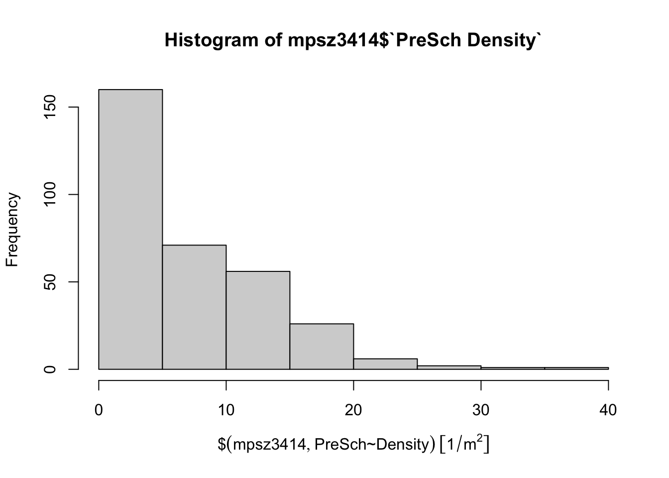

We improvef this graph by using ggplot.

ggplot(data=mpsz3414, 
       aes(x= as.numeric(`PreSch Density`)))+
  geom_histogram(bins=20, 
                 color="black", 
                 fill="light blue") +
  labs(title = "Are pre-school even distributed in Singapore?",
       subtitle= "There are many planning sub-zones with a single pre-school, on the other hand, \nthere are a few sub-zones with at least 20 pre-schools",
      x = "Pre-school density (per km sq)",
      y = "Frequency")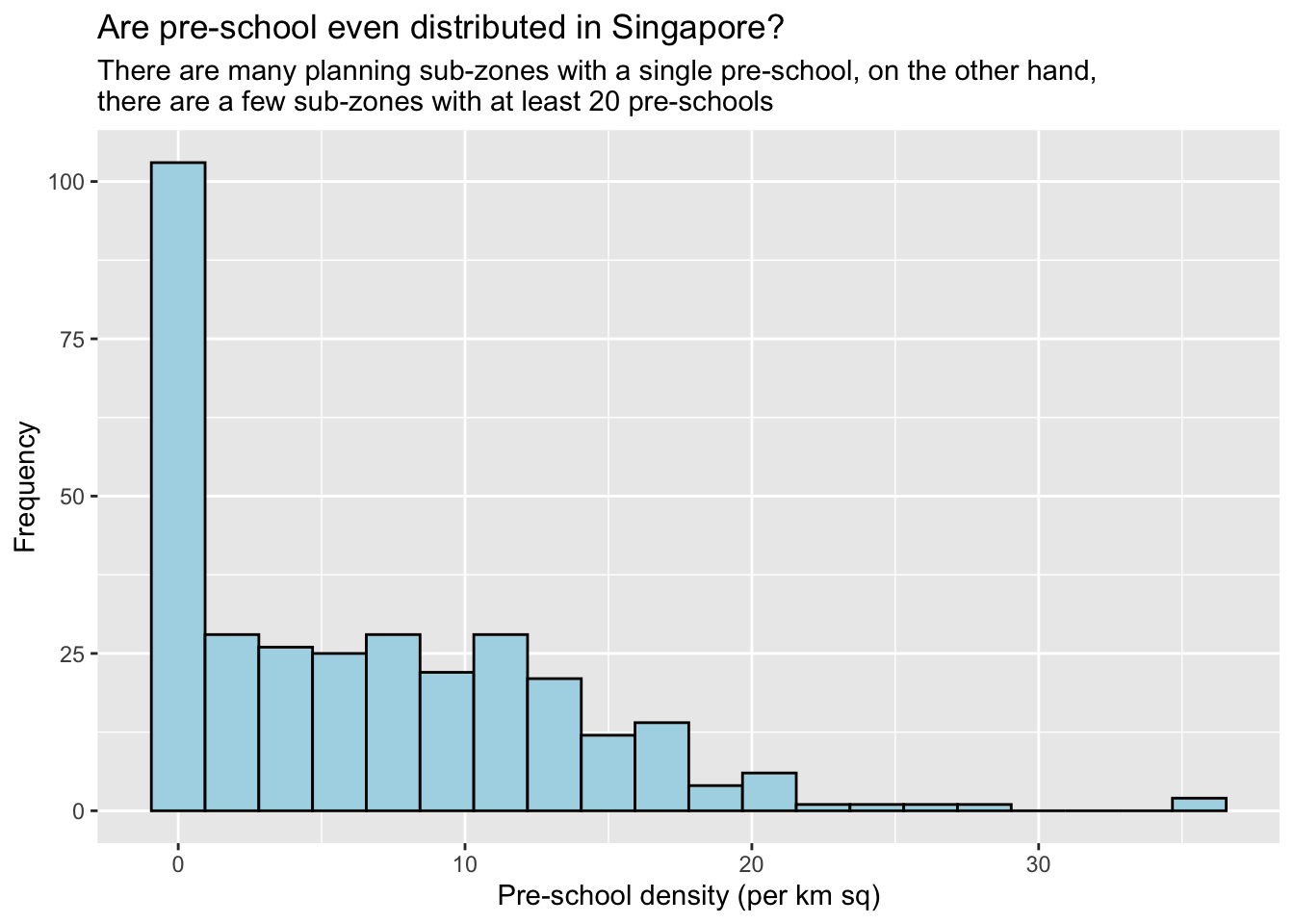

We can also create a scatter plot.

ggplot(data=mpsz3414, 
       aes(y = `PreSch Count`, 
           x= as.numeric(`PreSch Density`)))+
  geom_point(color="black", 
             fill="light blue") +
  xlim(0, 40) +
  ylim(0, 40) +
  labs(title = "",
      x = "Pre-school density (per km sq)",
      y = "Pre-school count")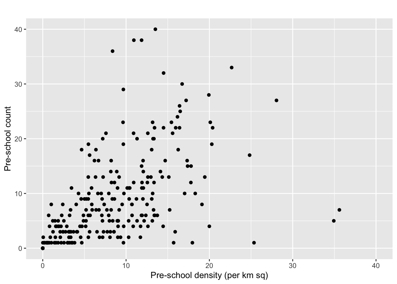

Others

Changing the website theme

After exploring Quarto docs, I found that we can change the theme. I decided on the zephyr theme as it looks most readable and aesthetic for me.

Issues with using Github on Rstudio

It was recommended to name the project with the convention <github_username>/ISSS624. However, due to restrictions on my machine, I had to deviate from this and create my project elsewhere.

Hence, I couldn’t use usethis::use_github() to setup my Github repository. However, as I use git Github intensively in my job, I did the setup manually myself to use the git functions on RStudio.

I used these steps for the manual setup.

Create the repo manually on Github on https://github.com/kjcpaas/ISSS624

Add the Github remote on RStudio project

> git remote add origin git@github.com:kjcpaas/ISSS624.git
> git remote -v
origin  git@github.com:kjcpaas/ISSS624.git (fetch)
origin  git@github.com:kjcpaas/ISSS624.git (push)

Set remote for head

> git remote set-head origin --auto
> git gc

After all these, I was able to use the git functions on RStudio.

Reflections

I thought it would be difficult to setup R and RStudio especially as the Cran Project site was down when I first attempted to set up. Good thing it was up the next day.
This course is looking to be very demanding indeed with a lot of time spent on pre-class assignments. However, I have enjoyed the hands-on exercise so far and I am eager to learn more!