In-class Ex 4: Geocoding

Setup Environment

httr - work with HTML pages

pacman::p_load(tidyverse, sf, httr, tmap)
tmap_mode("plot")
tmap_style("natural")

Geocoding

Use https://www.onemap.gov.sg/apidocs/

X, Y in SVY21, longitude latitude in WGS84

url <- "https://www.onemap.gov.sg/api/common/elastic/search"

csv <- read_csv("data/aspatial/GeneralInformationofschools.csv")
postcodes <- csv$"postal_code"

found <- data.frame()
not_found <- data.frame()

for(postcode in postcodes){
  query <- list("searchVal"=postcode,"returnGeom"="Y", "getAddrDetails"="Y","pageNum"="1")
  res<- GET(url, query=query)
  
  if((content(res)$found) !=0){
    found <- rbind(found, data.frame(content(res))[4:13])
  } else {
    not_found = data.frame(postcode)
  }
}

write_rds(found, "data/rds/found.rds")
write_rds(not_found, "data/rds/not_found.rds")

csv <- read_csv("data/aspatial/GeneralInformationofschools.csv")
found <- read_rds("data/rds/found.rds")
not_found <- read_rds("data/rds/not_found.rds")
merged = merge(csv, found, by.x = "postal_code", by.y = "results.POSTAL", all = TRUE)
write.csv(merged, file = "data/aspatial/schools.csv")
write.csv(not_found, file = "data/aspatial/not_found.csv")

Important

Use Google to look for the school without geospatial data.

Replace latitude with 1.3887, longitude with 103.7652.

Do this before proceeding to the next step. Or else st_as_sf() will complain about missing longitude and latitude

Preparation

Importing geocoded schools

• Import schools.csv

• Rename column names

• Retain only relevant columns

schools <- read_csv("data/aspatial/schools.csv") %>%
  rename(latitude = results.LATITUDE,
         longitude = results.LONGITUDE) %>%
  select(postal_code, school_name, latitude, longitude)

schools_sf <- st_as_sf(schools,
                       coords = c("longitude", "latitude"),
                       crs=4326) %>%
  st_transform(crs = 3414)

Confirming projection

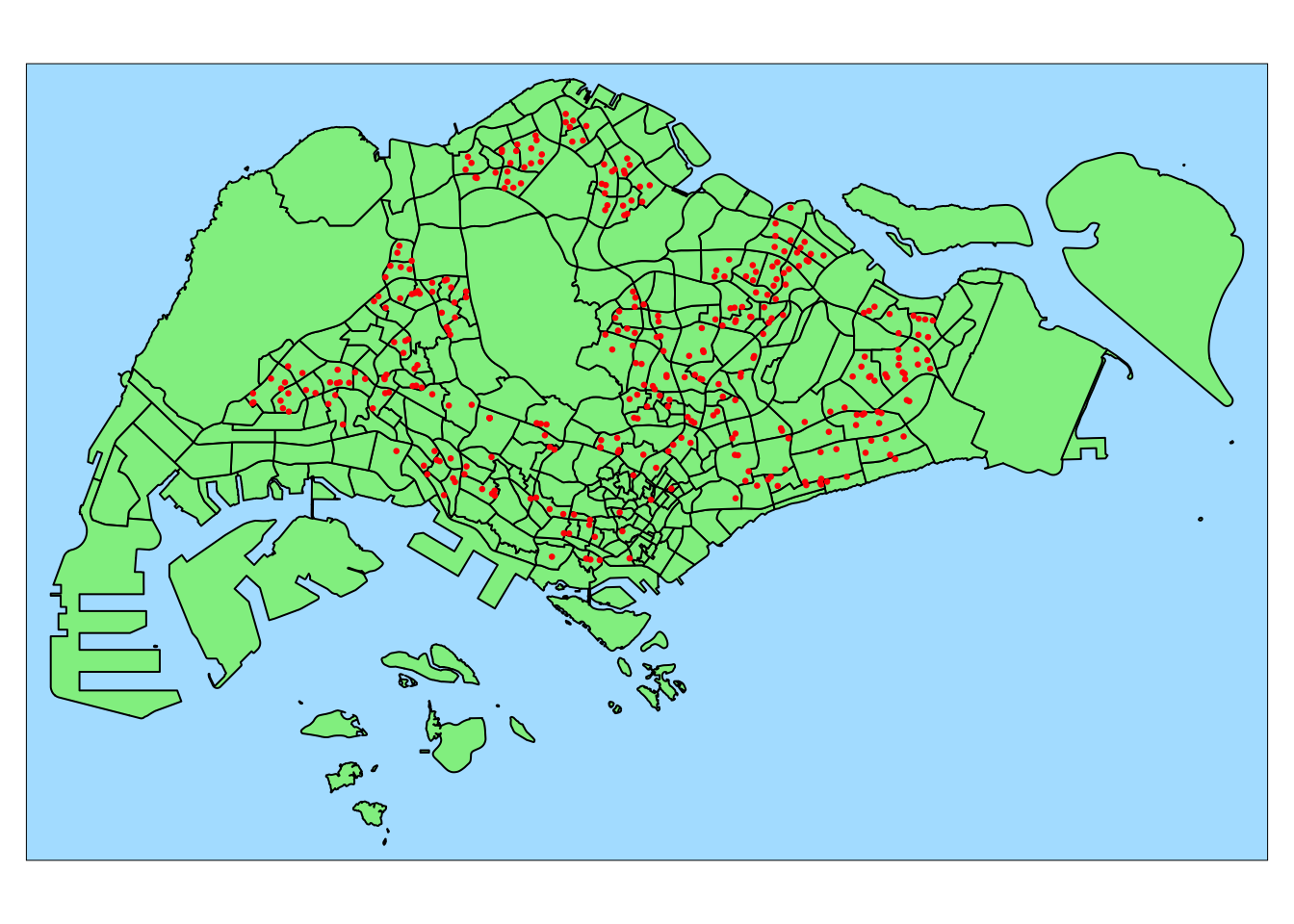
Note

I used the projected mpsz from previous exercises.

mpsz <- read_rds("data/rds/mpsz.rds")

tm_shape(mpsz) +
  tm_polygons(col = "lightgreen") +
  tm_shape(schools_sf) +
  tm_dots(col = "red", size = 0.025) #+

  #tm_view(set.zoom.limits = c(11, 14))

Finding how many schools per planning subzone using point in polygon count

mpsz$SCHOOL_COUNT <- lengths(st_intersects(mpsz, schools_sf))

Inspect the summary of statistics

summary(mpsz$SCHOOL_COUNT)

   Min. 1st Qu.  Median    Mean 3rd Qu.    Max. 
  0.000   0.000   0.000   1.054   2.000  12.000 

Importing business geospatial data

businesses <- st_read(dsn = "data/geospatial",
                      layer = "Business")

Reading layer `Business' from data source 
  `/Users/kjcpaas/Documents/Grad School/ISSS624/Project/ISSS624/In-class_Ex4/data/geospatial' 
  using driver `ESRI Shapefile'
Simple feature collection with 6550 features and 3 fields
Geometry type: POINT
Dimension:     XY
Bounding box:  xmin: 3669.148 ymin: 25408.41 xmax: 47034.83 ymax: 50148.54
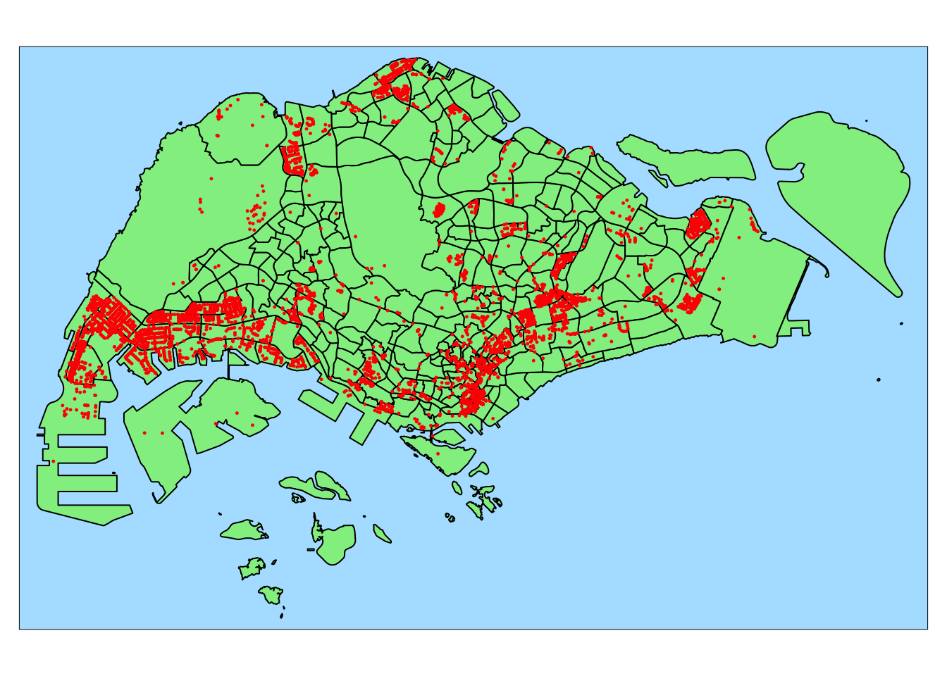
Projected CRS: SVY21 / Singapore TM

tmap_options(check.and.fix = TRUE)
tm_shape(mpsz) +
  tm_polygons(col = "lightgreen") +
  tm_shape(businesses) +
  tm_dots(col = "red", size = 0.01)

Data integration and wrangling

flow_data <- read_rds("data/rds/flow_data_tidy.rds")

# Check how to make this work
flow_data <- flow_data %>% left_join(mpsz, by= c("DESTIN_SZ", "SUBZONE_C"))