pacman::p_load(sf, spdep, tmap, tidyverse, knitr)Hands-on Exercise 2A: Spatial Weights and Applications
Overview
This hands-on exercise covers Chapter 8: Spatial Weights and Applications
I learned about the following:
- Calculating spatial weights
- Calculating spatially lagged variables
Getting Started
Preparing the data sets
Data sets used on this exercise were downloaded from E-learn.
Geospatial
- Hunan county boundary layer (
shpformat)
Aspatial
- Hunan’s local development indicators in 2012 (
csvformat)
Next, is putting them under the Hands-on_Ex2 directory, with the following file structure:
Hands-on_Ex2
└── data
    ├── aspatial
    │   └── Hunan_2012.csv
    └── geospatial
        ├── Hunan.dbf
        ├── Hunan.prj
        ├── Hunan.qpj
        ├── Hunan.shp
        └── Hunan.shx
Installing R packages
I used the code below to install the R packages used in the exercise:
Getting the Data Into R Environment
Importing data sets
I used st_read() to import the geospatial shp data.
hunan <- st_read(dsn = "data/geospatial",
                 layer = "Hunan")
Reading layer `Hunan' from data source
`/Users/kjcpaas/Documents/Grad School/ISSS624/Project/ISSS624/Hands-on_Ex2/data/geospatial'
using driver `ESRI Shapefile'
Simple feature collection with 88 features and 7 fields
Geometry type: POLYGON
Dimension: XY
Bounding box: xmin: 108.7831 ymin: 24.6342 xmax: 114.2544 ymax: 30.12812
Geodetic CRS: WGS 84In the previous exercises, we transformed the data with EPSG:3414. However, that is not applicable for this data set as we are not working with Singapore 🇸🇬 data set.
As with the previous exercises, I used read_csv() to import aspatial csv data.
hunan2012 <- read_csv("data/aspatial/Hunan_2012.csv")Joining the data sets
In the exercise, we have to join the 2 data sets using this code:
hunan <- left_join(hunan, hunan2012)%>%
select(1:4, 7, 15)We did not specify any columns to join by but left_join detected common column, County, so it joined the 2 data sets by this column.
At the end of this, we are left with 7 columns, which includes GDPPC from the aspatial data, which contains data for Gross Domestic Product per Capita.
Generating a quick thematic map
I used qtm() and other tmap functions to generate a map of the data.
basemap <- tm_shape(hunan) +
  tm_polygons() +
  tm_text("NAME_3", size=0.5)

gdppc <- qtm(hunan, "GDPPC")
tmap_arrange(basemap, gdppc, asp=1, ncol=2)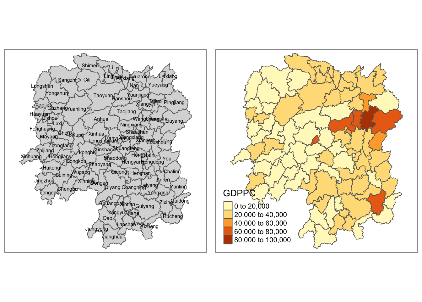
Maps do not need to be fancy at first. Using qtm() can already give us some useful insights and can guide us on how to proceed further with our analytics.
For example, from this map, I already see that the counties with the highest GDP per capital in the Central Eastern part of China, aside from a few exceptions.
Computing Contiguity Spatial Weights
This part makes use of poly2nb() to calculate the spatial weights.
Computing (QUEEN) contiguity based neighbors
wm_q <- poly2nb(hunan, queen=TRUE)
summary(wm_q)
Neighbour list object:
Number of regions: 88
Number of nonzero links: 448
Percentage nonzero weights: 5.785124
Average number of links: 5.090909
Link number distribution:
1 2 3 4 5 6 7 8 9 11
2 2 12 16 24 14 11 4 2 1
2 least connected regions:
30 65 with 1 link
1 most connected region:
85 with 11 linksThis showed that there are 2 least connected regions, 30 and 65. Furthermore, there is 1 county is most connected, 85.
Below I analyzed these counties of interest
Least connected counties
First, I checked the names of the least connected counties.
hunan$County[c(30, 65)][1] "Xinhuang" "Linxiang"The least connected counties are Xinhuang in the West and Linxiang in the Northeast.
It makes sense for these counties to be least connected as they are counties that only have 1 neighbors each, according to the map.
hunan$County[c(
  wm_q[[30]],
  wm_q[[65]]
)]
[1] "Zhijiang" "Yueyang" Xinhuang borders Zhijiang to the East, while Linxiang borders Yueyang to the Southwest.
Most connected county
hunan$County[85][1] "Taoyuan"The most connected county is Taoyuan with 11 neighbors. It’s neighbors are:
hunan$County[wm_q[[85]]] [1] "Anxiang" "Hanshou" "Jinshi" "Linli" "Shimen" "Yuanling"
[7] "Anhua" "Nan" "Cili" "Sangzhi" "Taojiang"This makes perfect sense as Taoyuan is a relatively large, inner county.
Creating (ROOK) contiguity based neighbors
wm_r <- poly2nb(hunan, queen=FALSE)
summary(wm_r)
Neighbour list object:
Number of regions: 88
Number of nonzero links: 440
Percentage nonzero weights: 5.681818
Average number of links: 5
Link number distribution:
1 2 3 4 5 6 7 8 9 10
2 2 12 20 21 14 11 3 2 1
2 least connected regions:
30 65 with 1 link
1 most connected region:
85 with 10 linksThis operation resulted in 8 fewer non-zero links. The most connected region, Taoyuan, has one less neighbor. However, the least connected regions stayed the same.
setdiff(hunan$County[wm_q[[85]]], hunan$County[wm_r[[85]]])[1] "Nan"Nan is not considered a neighbor of Taoyuan using the Rook method. I check the documentation of poly2nb() to understand why.
When setting queen=false, it requires boundaries to be more that just one point. On the other hand, with queen=true, it requires the objects to shared only a single point.
As such, having 8 less links means 8 pairs of counties only share a single point in their boundaries.
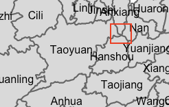
Looking at the map, Nan indeed only touches Taoyuan at a single point:
Visualising contiguity weights
To plot the contiguity, we need to get the centroids of each county region. To get this for a single county, the following code can be used.
hunan$geometry[1] %>% st_centroid(.x)Geometry set for 1 feature
Geometry type: POINT
Dimension: XY
Bounding box: xmin: 112.1531 ymin: 29.44346 xmax: 112.1531 ymax: 29.44346
Geodetic CRS: WGS 84However, we needed to plot each longitude and latitude separately and create a new data frame for centroid coordinates from those. In order to do that, I copied the code chunks from the exercise.
longitude <- map_dbl(hunan$geometry, ~st_centroid(.x)[[1]])
latitude <- map_dbl(hunan$geometry, ~st_centroid(.x)[[2]])
coords <- cbind(longitude, latitude)
head(coords)
longitude latitude
[1,] 112.1531 29.44362
[2,] 112.0372 28.86489
[3,] 111.8917 29.47107
[4,] 111.7031 29.74499
[5,] 111.6138 29.49258
[6,] 111.0341 29.79863Plotting contiguity based neighbors map
I plotted the Queen and Rooks maps on the same plot instead of the recommended way in the exercise. This is so I could see which neighbors where present in the Queen method but were not present in the Rook method.
They are the red lines in the map.
plot(hunan$geometry, border="lightgrey")
plot(wm_q, coords, pch = 19, cex = 0.6, add = TRUE, col= "red", main="Queen Contiguity")
plot(wm_r, coords, pch = 19, cex = 0.6, add = TRUE, col = "blue", main="Rook Contiguity")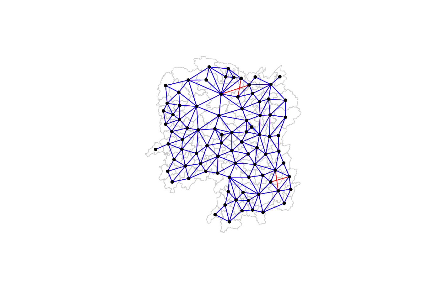
Computing distance-based neighbors
The data set uses WSG84 projection so distances are calculated according to this.
This part makes use of knearneigh() to calculate the spatial weights.
One observation is that a county’s nearest neighbor does not necessarily mean that said country is also the nearest neighbor of the neighboring country.
For example if B is the nearest neighbor of A, A may not be the nearest neighbor of B. B’s nearest neighbor might be another county, e.g., C.
See below for some examples.
knearneigh(coords)$nn[c(1,3,30,33,28,49)][1] 3 1 33 28 49 28In this example, 1 and 3 are nearest neighbors of each other. However, 30 is not 33’s nearest neighbor even though 33 is 30’s.
Determining cut-off distance
k1 <- knn2nb(knearneigh(coords))
k1dists <- unlist(nbdists(k1, coords, longlat = TRUE))
summary(k1dists)
Min. 1st Qu. Median Mean 3rd Qu. Max.
24.79 32.57 38.01 39.07 44.52 61.79 This means that the (centroids of) closest neighbors are 24.79 km apart while the farthest neighbors are 61.79 km apart.
To ensure that all counties will have at least one neighbors, we set the cut-off distance to the maximum distance, or 61.79 km.
Computing fixed distance weight matrix
To figure out the neighbors within the 62km distance (rounded out from the previous result), we use dnearneigh() .
wm_d62 <- dnearneigh(coords, 0, 62, longlat = TRUE)
wm_d62
Neighbour list object:
Number of regions: 88
Number of nonzero links: 324
Percentage nonzero weights: 4.183884
Average number of links: 3.681818 The average number of links here correspond to the average number of neighbors each county has.
That means for every county in China, there are 3.681818 other counties within 62 km of them, on average.
The example below gives a glimpse of neighbors each county has.
str(wm_d62)List of 88
$ : int [1:5] 3 4 5 57 64
$ : int [1:4] 57 58 78 85
$ : int [1:4] 1 4 5 57
$ : int [1:3] 1 3 5
$ : int [1:4] 1 3 4 85
$ : int 69
$ : int [1:2] 67 84
$ : int [1:4] 9 46 47 78
$ : int [1:4] 8 46 68 84
$ : int [1:4] 16 22 70 72
$ : int [1:3] 14 17 72
$ : int [1:5] 13 60 61 63 83
$ : int [1:4] 12 15 60 83
$ : int [1:2] 11 17
$ : int 13
$ : int [1:4] 10 17 22 83
$ : int [1:3] 11 14 16
$ : int [1:3] 20 22 63
$ : int [1:5] 20 21 73 74 82
$ : int [1:5] 18 19 21 22 82
$ : int [1:6] 19 20 35 74 82 86
$ : int [1:4] 10 16 18 20
$ : int [1:3] 41 77 82
$ : int [1:4] 25 28 31 54
$ : int [1:4] 24 28 33 81
$ : int [1:4] 27 33 42 81
$ : int [1:2] 26 29
$ : int [1:6] 24 25 33 49 52 54
$ : int [1:2] 27 37
$ : int 33
$ : int [1:2] 24 36
$ : int 50
$ : int [1:5] 25 26 28 30 81
$ : int [1:3] 36 45 80
$ : int [1:6] 21 41 46 47 80 82
$ : int [1:5] 31 34 45 56 80
$ : int [1:2] 29 42
$ : int [1:3] 44 77 79
$ : int [1:4] 40 42 43 81
$ : int [1:3] 39 45 79
$ : int [1:5] 23 35 45 79 82
$ : int [1:5] 26 37 39 43 81
$ : int [1:3] 39 42 44
$ : int [1:2] 38 43
$ : int [1:6] 34 36 40 41 79 80
$ : int [1:5] 8 9 35 47 86
$ : int [1:5] 8 35 46 80 86
$ : int [1:5] 50 51 52 53 55
$ : int [1:4] 28 51 52 54
$ : int [1:6] 32 48 51 52 54 55
$ : int [1:4] 48 49 50 52
$ : int [1:6] 28 48 49 50 51 54
$ : int [1:2] 48 55
$ : int [1:5] 24 28 49 50 52
$ : int [1:4] 48 50 53 75
$ : int 36
$ : int [1:5] 1 2 3 58 64
$ : int [1:5] 2 57 64 66 68
$ : int [1:3] 60 87 88
$ : int [1:4] 12 13 59 61
$ : int [1:5] 12 60 62 63 87
$ : int [1:4] 61 63 77 87
$ : int [1:5] 12 18 61 62 83
$ : int [1:4] 1 57 58 76
$ : int 76
$ : int [1:5] 58 67 68 76 84
$ : int [1:2] 7 66
$ : int [1:4] 9 58 66 84
$ : int [1:2] 6 75
$ : int [1:3] 10 72 73
$ : int [1:2] 73 74
$ : int [1:3] 10 11 70
$ : int [1:4] 19 70 71 74
$ : int [1:5] 19 21 71 73 86
$ : int [1:2] 55 69
$ : int [1:3] 64 65 66
$ : int [1:3] 23 38 62
$ : int [1:2] 2 8
$ : int [1:4] 38 40 41 45
$ : int [1:5] 34 35 36 45 47
$ : int [1:5] 25 26 33 39 42
$ : int [1:6] 19 20 21 23 35 41
$ : int [1:4] 12 13 16 63
$ : int [1:4] 7 9 66 68
$ : int [1:2] 2 5
$ : int [1:4] 21 46 47 74
$ : int [1:4] 59 61 62 88
$ : int [1:2] 59 87
- attr(*, "class")= chr "nb"
- attr(*, "region.id")= chr [1:88] "1" "2" "3" "4" ...
- attr(*, "call")= language dnearneigh(x = coords, d1 = 0, d2 = 62, longlat = TRUE)
- attr(*, "dnn")= num [1:2] 0 62
- attr(*, "bounds")= chr [1:2] "GE" "LE"
- attr(*, "nbtype")= chr "distance"
- attr(*, "sym")= logi TRUEAnother observation here is that Taoyuan, which had 11 contiguity-based neighbors, now only has 2 neighbors when using distance-based methods.
wm_d62[88][[1]]
[1] 59 87Plotting distance-based matrix
plot(hunan$geometry, border="lightgrey")
plot(wm_d62, coords, add=TRUE)
plot(k1, coords, add=TRUE, col="red", length=0.08)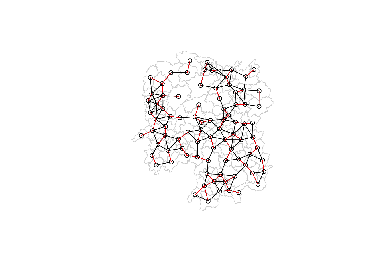
💡 I found out that plotting the red lines first before the black lines would just display black lines.
The technique of rendering the superset before the subset is a good technique to display the difference in the different plots.
After realizing this, I applied the same technique in the Queen and Rook maps in [##Visualising contiguity weights].
Computing adaptive distance weight matrix
There are cases in which knowing the k-nearest neighbors is useful. It can be done by passing k to knearneigh:
knn6 <- knn2nb(knearneigh(coords, k=6))
knn6
Neighbour list object:
Number of regions: 88
Number of nonzero links: 528
Percentage nonzero weights: 6.818182
Average number of links: 6
Non-symmetric neighbours listPlotting this in a map and overlapping with the wm_d62 map, we can see that more neighbor links (in red) were added so that each county has 6 neighbors.
plot(hunan$geometry, border="lightgrey")
plot(knn6, coords, add=TRUE, col="red", length=0.08)
plot(wm_d62, coords, add=TRUE)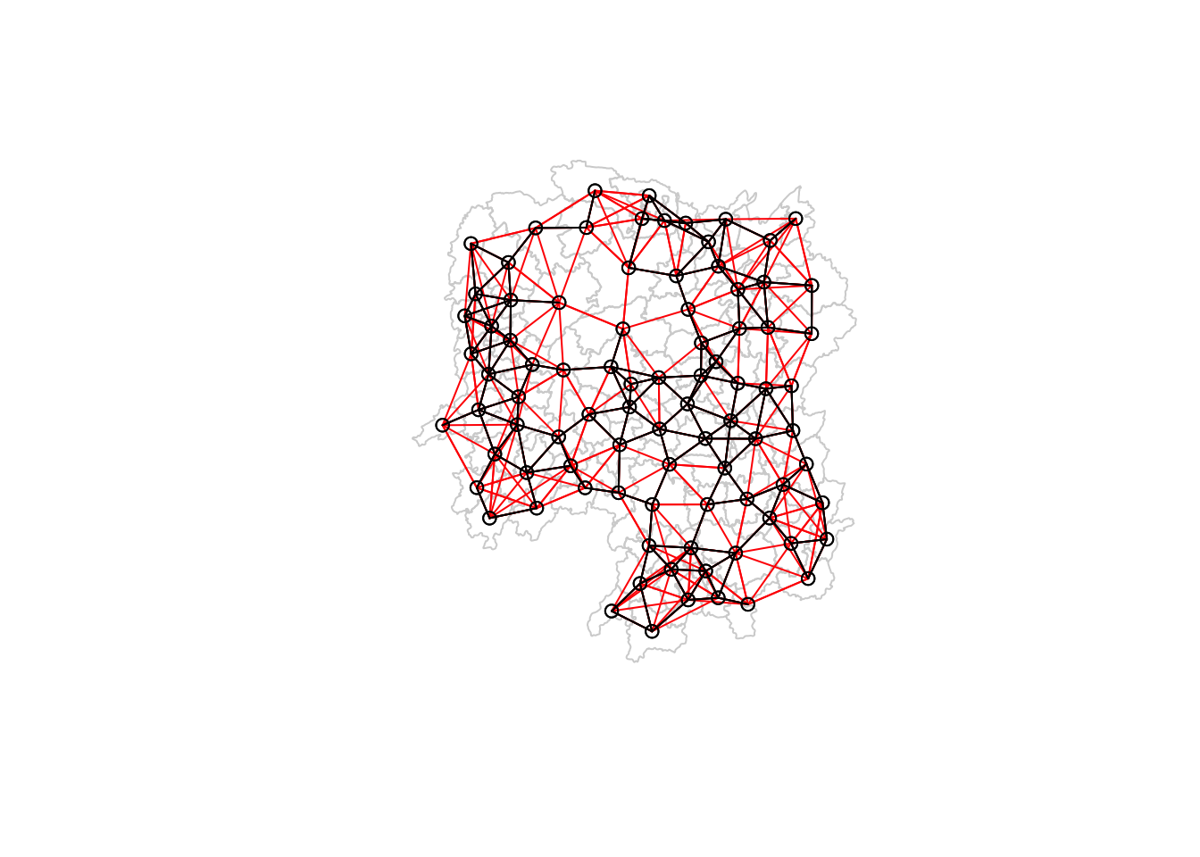
Weights based on IDW
Next I calculated inversed distance values. This is calculated by:
\[ 1/distance \]
In R, it can be obtained by:
dist <- nbdists(wm_q, coords, longlat = TRUE)
ids <- lapply(dist, function(x) 1/(x))
ids
[[1]]
[1] 0.01535405 0.03916350 0.01820896 0.02807922 0.01145113
[[2]]
[1] 0.01535405 0.01764308 0.01925924 0.02323898 0.01719350
[[3]]
[1] 0.03916350 0.02822040 0.03695795 0.01395765
[[4]]
[1] 0.01820896 0.02822040 0.03414741 0.01539065
[[5]]
[1] 0.03695795 0.03414741 0.01524598 0.01618354
[[6]]
[1] 0.015390649 0.015245977 0.021748129 0.011883901 0.009810297
[[7]]
[1] 0.01708612 0.01473997 0.01150924 0.01872915
[[8]]
[1] 0.02022144 0.03453056 0.02529256 0.01036340 0.02284457 0.01500600 0.01515314
[[9]]
[1] 0.02022144 0.01574888 0.02109502 0.01508028 0.02902705 0.01502980
[[10]]
[1] 0.02281552 0.01387777 0.01538326 0.01346650 0.02100510 0.02631658 0.01874863
[8] 0.01500046
[[11]]
[1] 0.01882869 0.02243492 0.02247473
[[12]]
[1] 0.02779227 0.02419652 0.02333385 0.02986130 0.02335429
[[13]]
[1] 0.02779227 0.02650020 0.02670323 0.01714243
[[14]]
[1] 0.01882869 0.01233868 0.02098555
[[15]]
[1] 0.02650020 0.01233868 0.01096284 0.01562226
[[16]]
[1] 0.02281552 0.02466962 0.02765018 0.01476814 0.01671430
[[17]]
[1] 0.01387777 0.02243492 0.02098555 0.01096284 0.02466962 0.01593341 0.01437996
[[18]]
[1] 0.02039779 0.02032767 0.01481665 0.01473691 0.01459380
[[19]]
[1] 0.01538326 0.01926323 0.02668415 0.02140253 0.01613589 0.01412874
[[20]]
[1] 0.01346650 0.02039779 0.01926323 0.01723025 0.02153130 0.01469240 0.02327034
[[21]]
[1] 0.02668415 0.01723025 0.01766299 0.02644986 0.02163800
[[22]]
[1] 0.02100510 0.02765018 0.02032767 0.02153130 0.01489296
[[23]]
[1] 0.01481665 0.01469240 0.01401432 0.02246233 0.01880425 0.01530458 0.01849605
[[24]]
[1] 0.02354598 0.01837201 0.02607264 0.01220154 0.02514180
[[25]]
[1] 0.02354598 0.02188032 0.01577283 0.01949232 0.02947957
[[26]]
[1] 0.02155798 0.01745522 0.02212108 0.02220532
[[27]]
[1] 0.02155798 0.02490625 0.01562326
[[28]]
[1] 0.01837201 0.02188032 0.02229549 0.03076171 0.02039506
[[29]]
[1] 0.02490625 0.01686587 0.01395022
[[30]]
[1] 0.02090587
[[31]]
[1] 0.02607264 0.01577283 0.01219005 0.01724850 0.01229012 0.01609781 0.01139438
[8] 0.01150130
[[32]]
[1] 0.01220154 0.01219005 0.01712515 0.01340413 0.01280928 0.01198216 0.01053374
[8] 0.01065655
[[33]]
[1] 0.01949232 0.01745522 0.02229549 0.02090587 0.01979045
[[34]]
[1] 0.03113041 0.03589551 0.02882915
[[35]]
[1] 0.01766299 0.02185795 0.02616766 0.02111721 0.02108253 0.01509020
[[36]]
[1] 0.01724850 0.03113041 0.01571707 0.01860991 0.02073549 0.01680129
[[37]]
[1] 0.01686587 0.02234793 0.01510990 0.01550676
[[38]]
[1] 0.01401432 0.02407426 0.02276151 0.01719415
[[39]]
[1] 0.01229012 0.02172543 0.01711924 0.02629732 0.01896385
[[40]]
[1] 0.01609781 0.01571707 0.02172543 0.01506473 0.01987922 0.01894207
[[41]]
[1] 0.02246233 0.02185795 0.02205991 0.01912542 0.01601083 0.01742892
[[42]]
[1] 0.02212108 0.01562326 0.01395022 0.02234793 0.01711924 0.01836831 0.01683518
[[43]]
[1] 0.01510990 0.02629732 0.01506473 0.01836831 0.03112027 0.01530782
[[44]]
[1] 0.01550676 0.02407426 0.03112027 0.01486508
[[45]]
[1] 0.03589551 0.01860991 0.01987922 0.02205991 0.02107101 0.01982700
[[46]]
[1] 0.03453056 0.04033752 0.02689769
[[47]]
[1] 0.02529256 0.02616766 0.04033752 0.01949145 0.02181458
[[48]]
[1] 0.02313819 0.03370576 0.02289485 0.01630057 0.01818085
[[49]]
[1] 0.03076171 0.02138091 0.02394529 0.01990000
[[50]]
[1] 0.01712515 0.02313819 0.02551427 0.02051530 0.02187179
[[51]]
[1] 0.03370576 0.02138091 0.02873854
[[52]]
[1] 0.02289485 0.02394529 0.02551427 0.02873854 0.03516672
[[53]]
[1] 0.01630057 0.01979945 0.01253977
[[54]]
[1] 0.02514180 0.02039506 0.01340413 0.01990000 0.02051530 0.03516672
[[55]]
[1] 0.01280928 0.01818085 0.02187179 0.01979945 0.01882298
[[56]]
[1] 0.01036340 0.01139438 0.01198216 0.02073549 0.01214479 0.01362855 0.01341697
[[57]]
[1] 0.028079221 0.017643082 0.031423501 0.029114131 0.013520292 0.009903702
[[58]]
[1] 0.01925924 0.03142350 0.02722997 0.01434859 0.01567192
[[59]]
[1] 0.01696711 0.01265572 0.01667105 0.01785036
[[60]]
[1] 0.02419652 0.02670323 0.01696711 0.02343040
[[61]]
[1] 0.02333385 0.01265572 0.02343040 0.02514093 0.02790764 0.01219751 0.02362452
[[62]]
[1] 0.02514093 0.02002219 0.02110260
[[63]]
[1] 0.02986130 0.02790764 0.01407043 0.01805987
[[64]]
[1] 0.02911413 0.01689892
[[65]]
[1] 0.02471705
[[66]]
[1] 0.01574888 0.01726461 0.03068853 0.01954805 0.01810569
[[67]]
[1] 0.01708612 0.01726461 0.01349843 0.01361172
[[68]]
[1] 0.02109502 0.02722997 0.03068853 0.01406357 0.01546511
[[69]]
[1] 0.02174813 0.01645838 0.01419926
[[70]]
[1] 0.02631658 0.01963168 0.02278487
[[71]]
[1] 0.01473997 0.01838483 0.03197403
[[72]]
[1] 0.01874863 0.02247473 0.01476814 0.01593341 0.01963168
[[73]]
[1] 0.01500046 0.02140253 0.02278487 0.01838483 0.01652709
[[74]]
[1] 0.01150924 0.01613589 0.03197403 0.01652709 0.01342099 0.02864567
[[75]]
[1] 0.011883901 0.010533736 0.012539774 0.018822977 0.016458383 0.008217581
[[76]]
[1] 0.01352029 0.01434859 0.01689892 0.02471705 0.01954805 0.01349843 0.01406357
[[77]]
[1] 0.014736909 0.018804247 0.022761507 0.012197506 0.020022195 0.014070428
[7] 0.008440896
[[78]]
[1] 0.02323898 0.02284457 0.01508028 0.01214479 0.01567192 0.01546511 0.01140779
[[79]]
[1] 0.01530458 0.01719415 0.01894207 0.01912542 0.01530782 0.01486508 0.02107101
[[80]]
[1] 0.01500600 0.02882915 0.02111721 0.01680129 0.01601083 0.01982700 0.01949145
[8] 0.01362855
[[81]]
[1] 0.02947957 0.02220532 0.01150130 0.01979045 0.01896385 0.01683518
[[82]]
[1] 0.02327034 0.02644986 0.01849605 0.02108253 0.01742892
[[83]]
[1] 0.023354289 0.017142433 0.015622258 0.016714303 0.014379961 0.014593799
[7] 0.014892965 0.018059871 0.008440896
[[84]]
[1] 0.01872915 0.02902705 0.01810569 0.01361172 0.01342099 0.01297994
[[85]]
[1] 0.011451133 0.017193502 0.013957649 0.016183544 0.009810297 0.010656545
[7] 0.013416965 0.009903702 0.014199260 0.008217581 0.011407794
[[86]]
[1] 0.01515314 0.01502980 0.01412874 0.02163800 0.01509020 0.02689769 0.02181458
[8] 0.02864567 0.01297994
[[87]]
[1] 0.01667105 0.02362452 0.02110260 0.02058034
[[88]]
[1] 0.01785036 0.02058034Row-standardized weights matrix
Next we assign the weight of 1/(# of neighbors) to each neighbor.
rswm_q <- nb2listw(wm_q, style="W", zero.policy = TRUE)
rswm_q
Characteristics of weights list object:
Neighbour list object:
Number of regions: 88
Number of nonzero links: 448
Percentage nonzero weights: 5.785124
Average number of links: 5.090909
Weights style: W
Weights constants summary:
n nn S0 S1 S2
W 88 7744 88 37.86334 365.9147Next I inspected some weights values to check if the results are consistent with our expectations.
rswm_q$weights[c(1, 10, 30, 85)][[1]]
[1] 0.2 0.2 0.2 0.2 0.2
[[2]]
[1] 0.125 0.125 0.125 0.125 0.125 0.125 0.125 0.125
[[3]]
[1] 1
[[4]]
[1] 0.09090909 0.09090909 0.09090909 0.09090909 0.09090909 0.09090909
[7] 0.09090909 0.09090909 0.09090909 0.09090909 0.09090909As expected, their values are equal to 1/(# of neighbors).
Next, the same was also done to derive a row standardised distance weight matrix.
rswm_ids <- nb2listw(wm_q, glist=ids, style="B", zero.policy=TRUE)
rswm_ids
Characteristics of weights list object:
Neighbour list object:
Number of regions: 88
Number of nonzero links: 448
Percentage nonzero weights: 5.785124
Average number of links: 5.090909
Weights style: B
Weights constants summary:
n nn S0 S1 S2
B 88 7744 8.786867 0.3776535 3.8137Checking some of the matrix values:
rswm_ids$weights[c(1, 10, 30, 85)][[1]]
[1] 0.01535405 0.03916350 0.01820896 0.02807922 0.01145113
[[2]]
[1] 0.02281552 0.01387777 0.01538326 0.01346650 0.02100510 0.02631658 0.01874863
[8] 0.01500046
[[3]]
[1] 0.02090587
[[4]]
[1] 0.011451133 0.017193502 0.013957649 0.016183544 0.009810297 0.010656545
[7] 0.013416965 0.009903702 0.014199260 0.008217581 0.011407794Results seem to be the same as when using nbdists() and lapply() in Weights based on IDW.
Finally, we get some summary of the values.
summary(unlist(rswm_ids$weights)) Min. 1st Qu. Median Mean 3rd Qu. Max.
0.008218 0.015088 0.018739 0.019614 0.022823 0.040338 Application of Spatial Weight Matrix
Spatial lag with row-standardized weights
First, I computed the spatially lagged values for each polygon.
GDPPC.lag <- lag.listw(rswm_q, hunan$GDPPC)
GDPPC.lag
[1] 24847.20 22724.80 24143.25 27737.50 27270.25 21248.80 43747.00 33582.71
[9] 45651.17 32027.62 32671.00 20810.00 25711.50 30672.33 33457.75 31689.20
[17] 20269.00 23901.60 25126.17 21903.43 22718.60 25918.80 20307.00 20023.80
[25] 16576.80 18667.00 14394.67 19848.80 15516.33 20518.00 17572.00 15200.12
[33] 18413.80 14419.33 24094.50 22019.83 12923.50 14756.00 13869.80 12296.67
[41] 15775.17 14382.86 11566.33 13199.50 23412.00 39541.00 36186.60 16559.60
[49] 20772.50 19471.20 19827.33 15466.80 12925.67 18577.17 14943.00 24913.00
[57] 25093.00 24428.80 17003.00 21143.75 20435.00 17131.33 24569.75 23835.50
[65] 26360.00 47383.40 55157.75 37058.00 21546.67 23348.67 42323.67 28938.60
[73] 25880.80 47345.67 18711.33 29087.29 20748.29 35933.71 15439.71 29787.50
[81] 18145.00 21617.00 29203.89 41363.67 22259.09 44939.56 16902.00 16930.00The spatially lagged GDPPC values were appended to the Hunan data using the code below:
lag.list <- list(hunan$NAME_3, lag.listw(rswm_q, hunan$GDPPC))
lag.res <- as.data.frame(lag.list)
colnames(lag.res) <- c("NAME_3", "lag GDPPC")
hunan <- left_join(hunan,lag.res)
head(hunan)
Simple feature collection with 6 features and 7 fields
Geometry type: POLYGON
Dimension: XY
Bounding box: xmin: 110.4922 ymin: 28.61762 xmax: 112.3013 ymax: 30.12812
Geodetic CRS: WGS 84
NAME_2 ID_3 NAME_3 ENGTYPE_3 County GDPPC lag GDPPC
1 Changde 21098 Anxiang County Anxiang 23667 24847.20
2 Changde 21100 Hanshou County Hanshou 20981 22724.80
3 Changde 21101 Jinshi County City Jinshi 34592 24143.25
4 Changde 21102 Li County Li 24473 27737.50
5 Changde 21103 Linli County Linli 25554 27270.25
6 Changde 21104 Shimen County Shimen 27137 21248.80
geometry
1 POLYGON ((112.0625 29.75523...
2 POLYGON ((112.2288 29.11684...
3 POLYGON ((111.8927 29.6013,...
4 POLYGON ((111.3731 29.94649...
5 POLYGON ((111.6324 29.76288...
6 POLYGON ((110.8825 30.11675...Next, the GDPPC and spatial lag GDPPC were plotted for comparison
gdppc <- qtm(hunan, "GDPPC")
lag_gdppc <- qtm(hunan, "lag GDPPC")
tmap_arrange(gdppc, lag_gdppc, asp=1, ncol=2)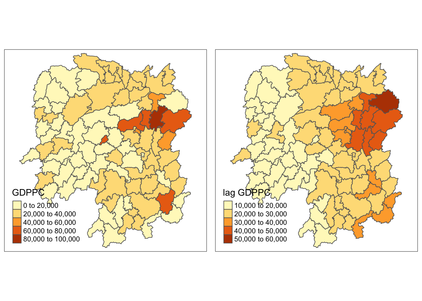
The spatial correlation seems to appear more positive among counties in the East.
Spatial lag as a sum of neighboring values
The spatial lag as a sum of neighboring values was calculated by assigning binary weights.
b_weights <- lapply(wm_q, function(x) 0*x + 1)
b_weights2 <- nb2listw(wm_q,
                       glist = b_weights,
                       style = "B")
b_weights2
Characteristics of weights list object:
Neighbour list object:
Number of regions: 88
Number of nonzero links: 448
Percentage nonzero weights: 5.785124
Average number of links: 5.090909
Weights style: B
Weights constants summary:
n nn S0 S1 S2
B 88 7744 448 896 10224Then, these weights were applied to the GDPPC values, and appending the lag_sum data to thehunan data set.
lag_sum <- list(hunan$NAME_3, lag.listw(b_weights2, hunan$GDPPC))
lag.res <- as.data.frame(lag_sum)
colnames(lag.res) <- c("NAME_3", "lag_sum GDPPC")
hunan <- left_join(hunan, lag.res)
Lastly, I plotted the map.
gdppc <- qtm(hunan, "GDPPC")
lag_sum_gdppc <- qtm(hunan, "lag_sum GDPPC")
tmap_arrange(gdppc, lag_sum_gdppc, asp=1, ncol=2)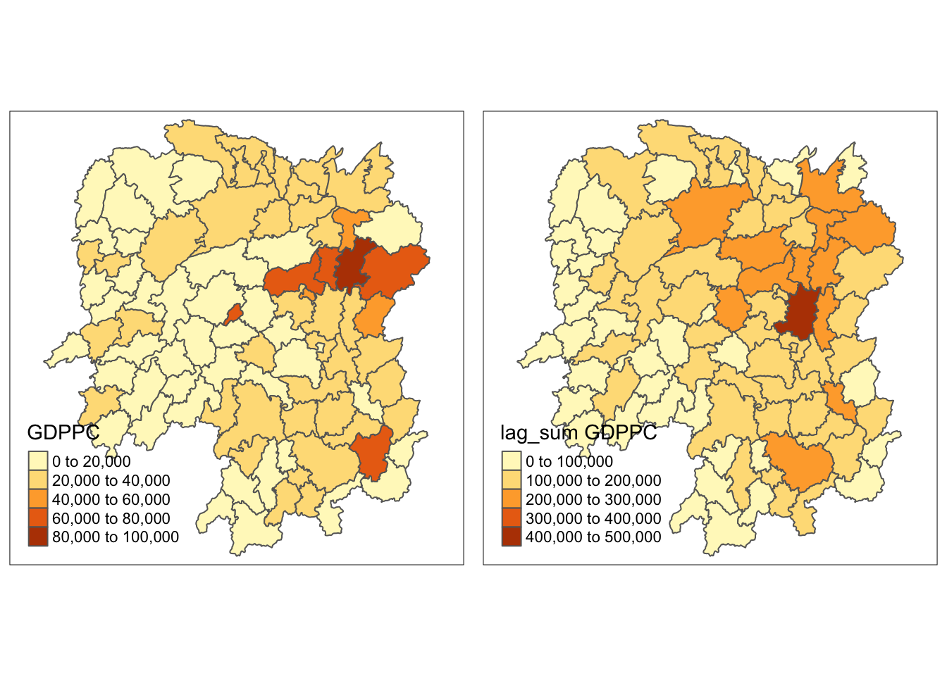
The lag_sum plot looks more scattered compared to the lag plot.
Spatial window average
First, I added the diagonal element to the neighbor list.
wm_qs <- include.self(wm_q)Next, I calculated the weights for the new list.
wm_qs <- nb2listw(wm_qs)
wm_qs
Characteristics of weights list object:
Neighbour list object:
Number of regions: 88
Number of nonzero links: 536
Percentage nonzero weights: 6.921488
Average number of links: 6.090909
Weights style: W
Weights constants summary:
n nn S0 S1 S2
W 88 7744 88 30.90265 357.5308Then, I creates the lag variable from the weight structure and GDPPC variable.
lag_w_avg_gpdpc <- lag.listw(wm_qs, hunan$GDPPC)
lag_w_avg_gpdpc
[1] 24650.50 22434.17 26233.00 27084.60 26927.00 22230.17 47621.20 37160.12
[9] 49224.71 29886.89 26627.50 22690.17 25366.40 25825.75 30329.00 32682.83
[17] 25948.62 23987.67 25463.14 21904.38 23127.50 25949.83 20018.75 19524.17
[25] 18955.00 17800.40 15883.00 18831.33 14832.50 17965.00 17159.89 16199.44
[33] 18764.50 26878.75 23188.86 20788.14 12365.20 15985.00 13764.83 11907.43
[41] 17128.14 14593.62 11644.29 12706.00 21712.29 43548.25 35049.00 16226.83
[49] 19294.40 18156.00 19954.75 18145.17 12132.75 18419.29 14050.83 23619.75
[57] 24552.71 24733.67 16762.60 20932.60 19467.75 18334.00 22541.00 26028.00
[65] 29128.50 46569.00 47576.60 36545.50 20838.50 22531.00 42115.50 27619.00
[73] 27611.33 44523.29 18127.43 28746.38 20734.50 33880.62 14716.38 28516.22
[81] 18086.14 21244.50 29568.80 48119.71 22310.75 43151.60 17133.40 17009.33Subsequently, I processed the data for further analysis.
lag.list.wm_qs <- list(hunan$NAME_3, lag.listw(wm_qs, hunan$GDPPC))
lag_wm_qs.res <- as.data.frame(lag.list.wm_qs)
colnames(lag_wm_qs.res) <- c("NAME_3", "lag_window_avg GDPPC")
hunan <- left_join(hunan, lag_wm_qs.res)
I inspected the different lag values to figure out if there was any pattern. It was hard to do by eye on this table.
hunan %>%
  select("County", "lag GDPPC", "lag_window_avg GDPPC") %>%
kable()| County | lag GDPPC | lag_window_avg GDPPC | geometry |
|---|---|---|---|
| Anxiang | 24847.20 | 24650.50 | POLYGON ((112.0625 29.75523… |
| Hanshou | 22724.80 | 22434.17 | POLYGON ((112.2288 29.11684… |
| Jinshi | 24143.25 | 26233.00 | POLYGON ((111.8927 29.6013,… |
| Li | 27737.50 | 27084.60 | POLYGON ((111.3731 29.94649… |
| Linli | 27270.25 | 26927.00 | POLYGON ((111.6324 29.76288… |
| Shimen | 21248.80 | 22230.17 | POLYGON ((110.8825 30.11675… |
| Liuyang | 43747.00 | 47621.20 | POLYGON ((113.9905 28.5682,… |
| Ningxiang | 33582.71 | 37160.12 | POLYGON ((112.7181 28.38299… |
| Wangcheng | 45651.17 | 49224.71 | POLYGON ((112.7914 28.52688… |
| Anren | 32027.62 | 29886.89 | POLYGON ((113.1757 26.82734… |
| Guidong | 32671.00 | 26627.50 | POLYGON ((114.1799 26.20117… |
| Jiahe | 20810.00 | 22690.17 | POLYGON ((112.4425 25.74358… |
| Linwu | 25711.50 | 25366.40 | POLYGON ((112.5914 25.55143… |
| Rucheng | 30672.33 | 25825.75 | POLYGON ((113.6759 25.87578… |
| Yizhang | 33457.75 | 30329.00 | POLYGON ((113.2621 25.68394… |
| Yongxing | 31689.20 | 32682.83 | POLYGON ((113.3169 26.41843… |
| Zixing | 20269.00 | 25948.62 | POLYGON ((113.7311 26.16259… |
| Changning | 23901.60 | 23987.67 | POLYGON ((112.6144 26.60198… |
| Hengdong | 25126.17 | 25463.14 | POLYGON ((113.1056 27.21007… |
| Hengnan | 21903.43 | 21904.38 | POLYGON ((112.7599 26.98149… |
| Hengshan | 22718.60 | 23127.50 | POLYGON ((112.607 27.4689, … |
| Leiyang | 25918.80 | 25949.83 | POLYGON ((112.9996 26.69276… |
| Qidong | 20307.00 | 20018.75 | POLYGON ((111.7818 27.0383,… |
| Chenxi | 20023.80 | 19524.17 | POLYGON ((110.2624 28.21778… |
| Zhongfang | 16576.80 | 18955.00 | POLYGON ((109.9431 27.72858… |
| Huitong | 18667.00 | 17800.40 | POLYGON ((109.9419 27.10512… |
| Jingzhou | 14394.67 | 15883.00 | POLYGON ((109.8186 26.75842… |
| Mayang | 19848.80 | 18831.33 | POLYGON ((109.795 27.98008,… |
| Tongdao | 15516.33 | 14832.50 | POLYGON ((109.9294 26.46561… |
| Xinhuang | 20518.00 | 17965.00 | POLYGON ((109.227 27.43733,… |
| Xupu | 17572.00 | 17159.89 | POLYGON ((110.7189 28.30485… |
| Yuanling | 15200.12 | 16199.44 | POLYGON ((110.9652 28.99895… |
| Zhijiang | 18413.80 | 18764.50 | POLYGON ((109.8818 27.60661… |
| Lengshuijiang | 14419.33 | 26878.75 | POLYGON ((111.5307 27.81472… |
| Shuangfeng | 24094.50 | 23188.86 | POLYGON ((112.263 27.70421,… |
| Xinhua | 22019.83 | 20788.14 | POLYGON ((111.3345 28.19642… |
| Chengbu | 12923.50 | 12365.20 | POLYGON ((110.4455 26.69317… |
| Dongan | 14756.00 | 15985.00 | POLYGON ((111.4531 26.86812… |
| Dongkou | 13869.80 | 13764.83 | POLYGON ((110.6622 27.37305… |
| Longhui | 12296.67 | 11907.43 | POLYGON ((110.985 27.65983,… |
| Shaodong | 15775.17 | 17128.14 | POLYGON ((111.9054 27.40254… |
| Suining | 14382.86 | 14593.62 | POLYGON ((110.389 27.10006,… |
| Wugang | 11566.33 | 11644.29 | POLYGON ((110.9878 27.03345… |
| Xinning | 13199.50 | 12706.00 | POLYGON ((111.0736 26.84627… |
| Xinshao | 23412.00 | 21712.29 | POLYGON ((111.6013 27.58275… |
| Shaoshan | 39541.00 | 43548.25 | POLYGON ((112.5391 27.97742… |
| Xiangxiang | 36186.60 | 35049.00 | POLYGON ((112.4549 28.05783… |
| Baojing | 16559.60 | 16226.83 | POLYGON ((109.7015 28.82844… |
| Fenghuang | 20772.50 | 19294.40 | POLYGON ((109.5239 28.19206… |
| Guzhang | 19471.20 | 18156.00 | POLYGON ((109.8968 28.74034… |
| Huayuan | 19827.33 | 19954.75 | POLYGON ((109.5647 28.61712… |
| Jishou | 15466.80 | 18145.17 | POLYGON ((109.8375 28.4696,… |
| Longshan | 12925.67 | 12132.75 | POLYGON ((109.6337 29.62521… |
| Luxi | 18577.17 | 18419.29 | POLYGON ((110.1067 28.41835… |
| Yongshun | 14943.00 | 14050.83 | POLYGON ((110.0003 29.29499… |
| Anhua | 24913.00 | 23619.75 | POLYGON ((111.6034 28.63716… |
| Nan | 25093.00 | 24552.71 | POLYGON ((112.3232 29.46074… |
| Yuanjiang | 24428.80 | 24733.67 | POLYGON ((112.4391 29.1791,… |
| Jianghua | 17003.00 | 16762.60 | POLYGON ((111.6461 25.29661… |
| Lanshan | 21143.75 | 20932.60 | POLYGON ((112.2286 25.61123… |
| Ningyuan | 20435.00 | 19467.75 | POLYGON ((112.0715 26.09892… |
| Shuangpai | 17131.33 | 18334.00 | POLYGON ((111.8864 26.11957… |
| Xintian | 24569.75 | 22541.00 | POLYGON ((112.2578 26.0796,… |
| Huarong | 23835.50 | 26028.00 | POLYGON ((112.9242 29.69134… |
| Linxiang | 26360.00 | 29128.50 | POLYGON ((113.5502 29.67418… |
| Miluo | 47383.40 | 46569.00 | POLYGON ((112.9902 29.02139… |
| Pingjiang | 55157.75 | 47576.60 | POLYGON ((113.8436 29.06152… |
| Xiangyin | 37058.00 | 36545.50 | POLYGON ((112.9173 28.98264… |
| Cili | 21546.67 | 20838.50 | POLYGON ((110.8822 29.69017… |
| Chaling | 23348.67 | 22531.00 | POLYGON ((113.7666 27.10573… |
| Liling | 42323.67 | 42115.50 | POLYGON ((113.5673 27.94346… |
| Yanling | 28938.60 | 27619.00 | POLYGON ((113.9292 26.6154,… |
| You | 25880.80 | 27611.33 | POLYGON ((113.5879 27.41324… |
| Zhuzhou | 47345.67 | 44523.29 | POLYGON ((113.2493 28.02411… |
| Sangzhi | 18711.33 | 18127.43 | POLYGON ((110.556 29.40543,… |
| Yueyang | 29087.29 | 28746.38 | POLYGON ((113.343 29.61064,… |
| Qiyang | 20748.29 | 20734.50 | POLYGON ((111.5563 26.81318… |
| Taojiang | 35933.71 | 33880.62 | POLYGON ((112.0508 28.67265… |
| Shaoyang | 15439.71 | 14716.38 | POLYGON ((111.5013 27.30207… |
| Lianyuan | 29787.50 | 28516.22 | POLYGON ((111.6789 28.02946… |
| Hongjiang | 18145.00 | 18086.14 | POLYGON ((110.1441 27.47513… |
| Hengyang | 21617.00 | 21244.50 | POLYGON ((112.7144 26.98613… |
| Guiyang | 29203.89 | 29568.80 | POLYGON ((113.0811 26.04963… |
| Changsha | 41363.67 | 48119.71 | POLYGON ((112.9421 28.03722… |
| Taoyuan | 22259.09 | 22310.75 | POLYGON ((112.0612 29.32855… |
| Xiangtan | 44939.56 | 43151.60 | POLYGON ((113.0426 27.8942,… |
| Dao | 16902.00 | 17133.40 | POLYGON ((111.498 25.81679,… |
| Jiangyong | 16930.00 | 17009.33 | POLYGON ((111.3659 25.39472… |
After all the data processing, I could finally plot the spatial window average.
w_avg_gdppc <- qtm(hunan, "lag_window_avg GDPPC")
tmap_arrange(lag_gdppc, w_avg_gdppc, asp=1, ncol=2)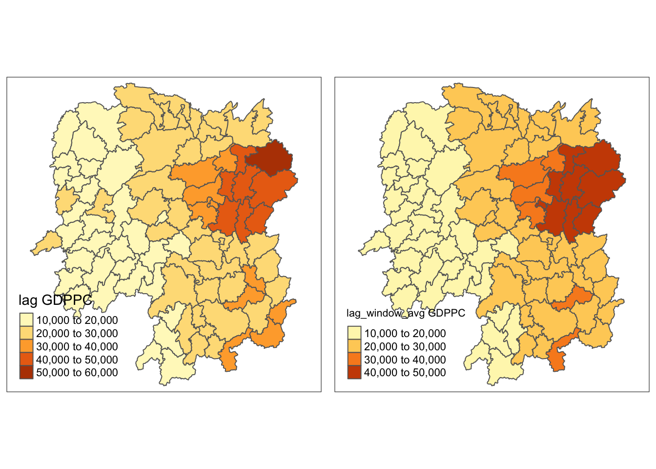
The range of values became narrower, from 10,000 - 60,000 to 10,000 - 50,000. Furthermore, the map looks “cleaner” for the lag_window_average.
Spatial window sum
First, I added the diagonal element to the neighbor list.
wm_qs <- include.self(wm_q)Then, binary weights were calculated from this new list.
b_weights <- lapply(wm_qs, function(x) 0*x + 1)
b_weights2 <- nb2listw(wm_qs,
                       glist = b_weights,
                       style = "B")
b_weights2
Characteristics of weights list object:
Neighbour list object:
Number of regions: 88
Number of nonzero links: 536
Percentage nonzero weights: 6.921488
Average number of links: 6.090909
Weights style: B
Weights constants summary:
n nn S0 S1 S2
B 88 7744 536 1072 14160w_sum_gdppc <- list(hunan$NAME_3, lag.listw(b_weights2, hunan$GDPPC))
w_sum_gdppc[[1]]
[1] "Anxiang" "Hanshou" "Jinshi" "Li"
[5] "Linli" "Shimen" "Liuyang" "Ningxiang"
[9] "Wangcheng" "Anren" "Guidong" "Jiahe"
[13] "Linwu" "Rucheng" "Yizhang" "Yongxing"
[17] "Zixing" "Changning" "Hengdong" "Hengnan"
[21] "Hengshan" "Leiyang" "Qidong" "Chenxi"
[25] "Zhongfang" "Huitong" "Jingzhou" "Mayang"
[29] "Tongdao" "Xinhuang" "Xupu" "Yuanling"
[33] "Zhijiang" "Lengshuijiang" "Shuangfeng" "Xinhua"
[37] "Chengbu" "Dongan" "Dongkou" "Longhui"
[41] "Shaodong" "Suining" "Wugang" "Xinning"
[45] "Xinshao" "Shaoshan" "Xiangxiang" "Baojing"
[49] "Fenghuang" "Guzhang" "Huayuan" "Jishou"
[53] "Longshan" "Luxi" "Yongshun" "Anhua"
[57] "Nan" "Yuanjiang" "Jianghua" "Lanshan"
[61] "Ningyuan" "Shuangpai" "Xintian" "Huarong"
[65] "Linxiang" "Miluo" "Pingjiang" "Xiangyin"
[69] "Cili" "Chaling" "Liling" "Yanling"
[73] "You" "Zhuzhou" "Sangzhi" "Yueyang"
[77] "Qiyang" "Taojiang" "Shaoyang" "Lianyuan"
[81] "Hongjiang" "Hengyang" "Guiyang" "Changsha"
[85] "Taoyuan" "Xiangtan" "Dao" "Jiangyong"
[[2]]
[1] 147903 134605 131165 135423 134635 133381 238106 297281 344573 268982
[11] 106510 136141 126832 103303 151645 196097 207589 143926 178242 175235
[21] 138765 155699 160150 117145 113730 89002 63532 112988 59330 35930
[31] 154439 145795 112587 107515 162322 145517 61826 79925 82589 83352
[41] 119897 116749 81510 63530 151986 174193 210294 97361 96472 108936
[51] 79819 108871 48531 128935 84305 188958 171869 148402 83813 104663
[61] 155742 73336 112705 78084 58257 279414 237883 219273 83354 90124
[71] 168462 165714 165668 311663 126892 229971 165876 271045 117731 256646
[81] 126603 127467 295688 336838 267729 431516 85667 51028Next, data was processed for further analysis.
w_sum_gdppc.res <- as.data.frame(w_sum_gdppc)
colnames(w_sum_gdppc.res) <- c("NAME_3", "w_sum GDPPC")
hunan <- left_join(hunan, w_sum_gdppc.res)
Next, I compared the lag_sum and w_sum values to check for patterns. Hard to see in this table format.
hunan %>%
  select("County", "lag_sum GDPPC", "w_sum GDPPC") %>%
kable()| County | lag_sum GDPPC | w_sum GDPPC | geometry |
|---|---|---|---|
| Anxiang | 124236 | 147903 | POLYGON ((112.0625 29.75523… |
| Hanshou | 113624 | 134605 | POLYGON ((112.2288 29.11684… |
| Jinshi | 96573 | 131165 | POLYGON ((111.8927 29.6013,… |
| Li | 110950 | 135423 | POLYGON ((111.3731 29.94649… |
| Linli | 109081 | 134635 | POLYGON ((111.6324 29.76288… |
| Shimen | 106244 | 133381 | POLYGON ((110.8825 30.11675… |
| Liuyang | 174988 | 238106 | POLYGON ((113.9905 28.5682,… |
| Ningxiang | 235079 | 297281 | POLYGON ((112.7181 28.38299… |
| Wangcheng | 273907 | 344573 | POLYGON ((112.7914 28.52688… |
| Anren | 256221 | 268982 | POLYGON ((113.1757 26.82734… |
| Guidong | 98013 | 106510 | POLYGON ((114.1799 26.20117… |
| Jiahe | 104050 | 136141 | POLYGON ((112.4425 25.74358… |
| Linwu | 102846 | 126832 | POLYGON ((112.5914 25.55143… |
| Rucheng | 92017 | 103303 | POLYGON ((113.6759 25.87578… |
| Yizhang | 133831 | 151645 | POLYGON ((113.2621 25.68394… |
| Yongxing | 158446 | 196097 | POLYGON ((113.3169 26.41843… |
| Zixing | 141883 | 207589 | POLYGON ((113.7311 26.16259… |
| Changning | 119508 | 143926 | POLYGON ((112.6144 26.60198… |
| Hengdong | 150757 | 178242 | POLYGON ((113.1056 27.21007… |
| Hengnan | 153324 | 175235 | POLYGON ((112.7599 26.98149… |
| Hengshan | 113593 | 138765 | POLYGON ((112.607 27.4689, … |
| Leiyang | 129594 | 155699 | POLYGON ((112.9996 26.69276… |
| Qidong | 142149 | 160150 | POLYGON ((111.7818 27.0383,… |
| Chenxi | 100119 | 117145 | POLYGON ((110.2624 28.21778… |
| Zhongfang | 82884 | 113730 | POLYGON ((109.9431 27.72858… |
| Huitong | 74668 | 89002 | POLYGON ((109.9419 27.10512… |
| Jingzhou | 43184 | 63532 | POLYGON ((109.8186 26.75842… |
| Mayang | 99244 | 112988 | POLYGON ((109.795 27.98008,… |
| Tongdao | 46549 | 59330 | POLYGON ((109.9294 26.46561… |
| Xinhuang | 20518 | 35930 | POLYGON ((109.227 27.43733,… |
| Xupu | 140576 | 154439 | POLYGON ((110.7189 28.30485… |
| Yuanling | 121601 | 145795 | POLYGON ((110.9652 28.99895… |
| Zhijiang | 92069 | 112587 | POLYGON ((109.8818 27.60661… |
| Lengshuijiang | 43258 | 107515 | POLYGON ((111.5307 27.81472… |
| Shuangfeng | 144567 | 162322 | POLYGON ((112.263 27.70421,… |
| Xinhua | 132119 | 145517 | POLYGON ((111.3345 28.19642… |
| Chengbu | 51694 | 61826 | POLYGON ((110.4455 26.69317… |
| Dongan | 59024 | 79925 | POLYGON ((111.4531 26.86812… |
| Dongkou | 69349 | 82589 | POLYGON ((110.6622 27.37305… |
| Longhui | 73780 | 83352 | POLYGON ((110.985 27.65983,… |
| Shaodong | 94651 | 119897 | POLYGON ((111.9054 27.40254… |
| Suining | 100680 | 116749 | POLYGON ((110.389 27.10006,… |
| Wugang | 69398 | 81510 | POLYGON ((110.9878 27.03345… |
| Xinning | 52798 | 63530 | POLYGON ((111.0736 26.84627… |
| Xinshao | 140472 | 151986 | POLYGON ((111.6013 27.58275… |
| Shaoshan | 118623 | 174193 | POLYGON ((112.5391 27.97742… |
| Xiangxiang | 180933 | 210294 | POLYGON ((112.4549 28.05783… |
| Baojing | 82798 | 97361 | POLYGON ((109.7015 28.82844… |
| Fenghuang | 83090 | 96472 | POLYGON ((109.5239 28.19206… |
| Guzhang | 97356 | 108936 | POLYGON ((109.8968 28.74034… |
| Huayuan | 59482 | 79819 | POLYGON ((109.5647 28.61712… |
| Jishou | 77334 | 108871 | POLYGON ((109.8375 28.4696,… |
| Longshan | 38777 | 48531 | POLYGON ((109.6337 29.62521… |
| Luxi | 111463 | 128935 | POLYGON ((110.1067 28.41835… |
| Yongshun | 74715 | 84305 | POLYGON ((110.0003 29.29499… |
| Anhua | 174391 | 188958 | POLYGON ((111.6034 28.63716… |
| Nan | 150558 | 171869 | POLYGON ((112.3232 29.46074… |
| Yuanjiang | 122144 | 148402 | POLYGON ((112.4391 29.1791,… |
| Jianghua | 68012 | 83813 | POLYGON ((111.6461 25.29661… |
| Lanshan | 84575 | 104663 | POLYGON ((112.2286 25.61123… |
| Ningyuan | 143045 | 155742 | POLYGON ((112.0715 26.09892… |
| Shuangpai | 51394 | 73336 | POLYGON ((111.8864 26.11957… |
| Xintian | 98279 | 112705 | POLYGON ((112.2578 26.0796,… |
| Huarong | 47671 | 78084 | POLYGON ((112.9242 29.69134… |
| Linxiang | 26360 | 58257 | POLYGON ((113.5502 29.67418… |
| Miluo | 236917 | 279414 | POLYGON ((112.9902 29.02139… |
| Pingjiang | 220631 | 237883 | POLYGON ((113.8436 29.06152… |
| Xiangyin | 185290 | 219273 | POLYGON ((112.9173 28.98264… |
| Cili | 64640 | 83354 | POLYGON ((110.8822 29.69017… |
| Chaling | 70046 | 90124 | POLYGON ((113.7666 27.10573… |
| Liling | 126971 | 168462 | POLYGON ((113.5673 27.94346… |
| Yanling | 144693 | 165714 | POLYGON ((113.9292 26.6154,… |
| You | 129404 | 165668 | POLYGON ((113.5879 27.41324… |
| Zhuzhou | 284074 | 311663 | POLYGON ((113.2493 28.02411… |
| Sangzhi | 112268 | 126892 | POLYGON ((110.556 29.40543,… |
| Yueyang | 203611 | 229971 | POLYGON ((113.343 29.61064,… |
| Qiyang | 145238 | 165876 | POLYGON ((111.5563 26.81318… |
| Taojiang | 251536 | 271045 | POLYGON ((112.0508 28.67265… |
| Shaoyang | 108078 | 117731 | POLYGON ((111.5013 27.30207… |
| Lianyuan | 238300 | 256646 | POLYGON ((111.6789 28.02946… |
| Hongjiang | 108870 | 126603 | POLYGON ((110.1441 27.47513… |
| Hengyang | 108085 | 127467 | POLYGON ((112.7144 26.98613… |
| Guiyang | 262835 | 295688 | POLYGON ((113.0811 26.04963… |
| Changsha | 248182 | 336838 | POLYGON ((112.9421 28.03722… |
| Taoyuan | 244850 | 267729 | POLYGON ((112.0612 29.32855… |
| Xiangtan | 404456 | 431516 | POLYGON ((113.0426 27.8942,… |
| Dao | 67608 | 85667 | POLYGON ((111.498 25.81679,… |
| Jiangyong | 33860 | 51028 | POLYGON ((111.3659 25.39472… |
Finally, I plotted the maps.
w_sum_gdppc <- qtm(hunan, "w_sum GDPPC")
tmap_arrange(lag_sum_gdppc, w_sum_gdppc, asp=1, ncol=2)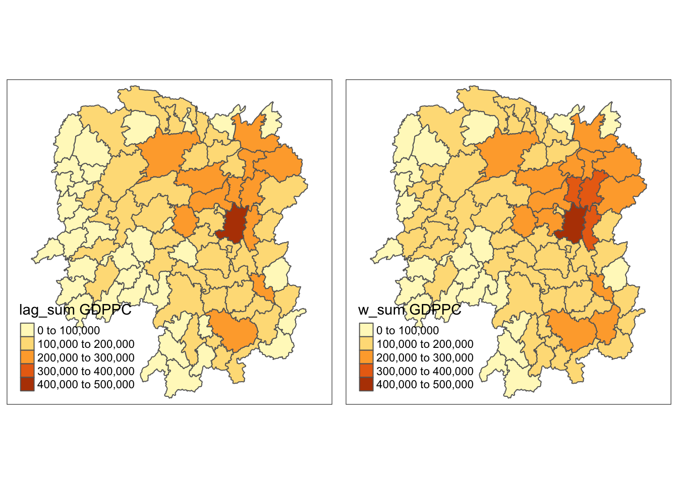
Reflections
This exercise was interesting for me as I used to develop simple games when I was learning how to code. I implemented some collision detection algorithm to figure out if balls need to bounce, or if a killed character needs to disappear from screen.
However, the logic I did before was very simple compared to what was done in this exercise as most elements in my games were simple geometric shapes like circle or rectangles.
I am interested to know more how these “collisions” are detected in geospatial analysis.